I’m currently teaching a Geometry course, and wished there was an easy way to illustrate geometric transformations for my students. I’m sure they’ll agree I’m not a great artist.
Since R is my preferred way to draw any picture, I thought “Let’s use GGPlot to show transformations!”
For those not versed in geometry, we would like to easily visualize translations (shifts along a vector), rotations, and dilations of points (or collections of points) in the complex plane. Reflections can be achieved via a combination of rotation and translation. Another important transformation, inversion, will be done in the next post.
Functions for the transformations
I’m going to write separate functions for the real and imaginary parts of the result of each transformation, this is to make things easy to produce dataframes to send to ggplot. There are more efficient ways to do this, but I want all functions to have a consistent input/output structure so applying transformations and graphing the results is easy.
Translations
Mathematically, a translation in the complex plane is a function that adds a fixed number to the input. The inputs tx and ty are the real and imaginary parts of the point we’re translating by.
translateR <- function(x,y,tx,ty){return (x+tx)}
translateI <- function(x,y,tx,ty){return (y+ty)}
Rotations and Dilations
Mathematically, multiplying by a complex number rotates (about the origin) by it’s argument and dilates by it’s modulus. Similarly to above, rx and ry are the real and imaginary parts of the number we multiply by to achieve the rotation/dilation (ry=0 will be just a dilation).
rotateR <- function(x,y,rx,ry){return (x*rx-y*ry)}
rotateI <- function(x,y,rx,ry){return (x*ry+y*rx)}
Rotations about a point other then the origin can be accomplished by applying a translation to the origin, rotation about the origin, and then translating back.
Illustrating the transformations
To clearly show a transformation, let’s start with a collection on points in the complex plane:
rectangle <- data.frame(x = c(rep(seq(from=0, to=2, by=.1),2), rep(0,11),rep(2,11)),
                  y=c(rep(0,21),rep(1,21),rep(seq(0,1,by=.1),2)))
rectangle$code <- "Original"

library(ggplot2)
ggplot(rectangle, aes(x=x,y=y))+geom_point(size=1)+xlim(c(-5,5))+ylim(c(-5,5))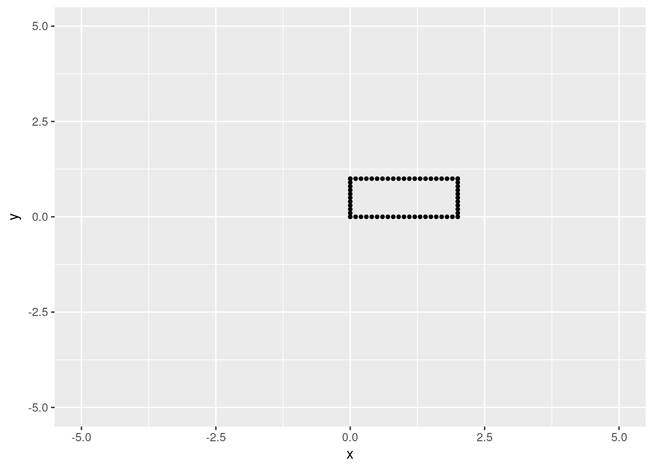
Now let’s try a translation by \(-1-2i\).
trRectangle <- data.frame(x = translateR(rectangle$x, rectangle$y, -1,-2),
                          y=translateI(rectangle$x, rectangle$y, -1,-2))
trRectangle$code <- "Translate"

library(dplyr)

rbind.data.frame(rectangle, trRectangle) %>%
  ggplot(aes(x=x,y=y,col=code))+geom_point(size=1)+
xlim(c(-5,5))+ylim(c(-5,5))![]()
And a rotation by \(\frac{2+3i}{\sqrt{13}}\) (why pick nice numbers?):
rotRectangle <- data.frame(x = rotateR(rectangle$x, rectangle$y, 2/sqrt(13),3/sqrt(13)),
y=rotateI(rectangle$x, rectangle$y, 2/sqrt(13),3/sqrt(13)))
rotRectangle$code <- "Rotation"
library(dplyr)
rbind.data.frame(rectangle, rotRectangle) %>%
ggplot(aes(x=x,y=y,col=code))+geom_point(size=1)+
xlim(c(-5,5))+ylim(c(-5,5))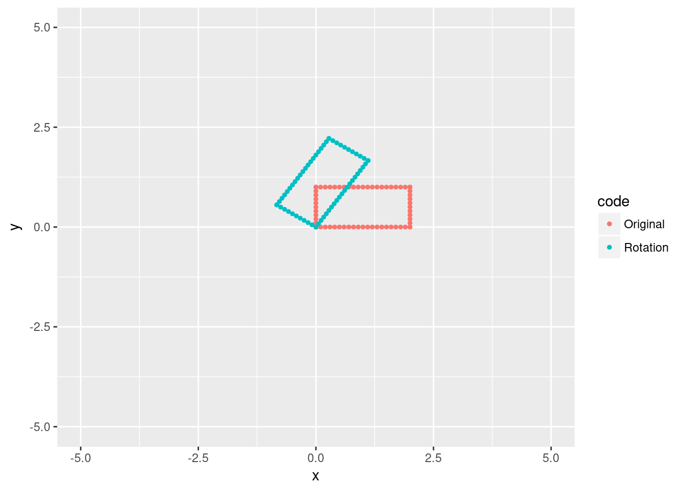 We can also perform more complicated transformations. Let’s rotate about the original rectangle’s top right corner \(2+i\) by \(\frac{\pi}{4}\), and double the size. This means we first move \((2,1)\) to the origin, rotate/dilate, then move back.
#translate to origin
glRect <- data.frame(x=translateR(rectangle$x, rectangle$y, -2,-1),
                     y=translateI(rectangle$x, rectangle$y, -2,-1))


#rotate and dilate by 2e^{i*pi/4} = sqrt(2)+isqrt(2)
#
#We're doing this in one line since both the real and imaginary
#rotations change and use the original coordinates. Two lines
#would produce very different transformation.
glRect[,1:2] <- c(rotateR(glRect$x, glRect$y, sqrt(2), sqrt(2)) ,
                  rotateI(glRect$x, glRect$y, sqrt(2),sqrt(2)))

#Now translate back
glRect$x <- translateR(glRect$x, glRect$y, 2,1)
glRect$y <- translateI(glRect$x, glRect$y, 2,1)

#add code for graph
glRect$code <-"Transformed"

#and graph
rbind.data.frame(rectangle, glRect) %>%
  ggplot(aes(x=x,y=y,col=code))+geom_point(size=1)+
xlim(c(-5,5))+ylim(c(-5,5))![]()
The combination of rotation and translation can also produce a reflection about any line.
Next up, inversions…