Introduction
Recently a student in another course came to my office looking for someone “who could explain the Monte Carlo simulation” to her. I was caught a bit off-guard since (a) it was 10 minutes before my geometry class and (b) there is no single Monte Carlo simulation.
After a brief discussion, I found out she wanted to predict stock prices using Monte Carlo simulation, but she thought that the Monte Carlo simulation provided the prediction - she couldn’t say how the actual predictions were being made which is the crucial part.
Aside on Monte Carlo
If you are familiar with Monte Carlo simulations, skip this, but if not it may be worth reading.
A Monte Carlo simulation is a process of using the outcomes of a random process to better understand the probability distribution of the process. The method of creating the outcomes if dependent on the situation (although it should utilize some type of random sampling).
In my Computer Science classes, I have students use a Monte Carlo simulation to calculate \(\pi\) (I usually do this Intro Stats too). This involves choosing \(x\) and \(y\) values between \(-1\) and \(1\) (uniform distribution) and seeing how many \((x,y)\) pairs are inside the unit circle. For a sufficiently large number of points, the ratio of the number inside to the total should be the same as the ratio of area of the unit circle to the area of the surrounding square (where all possible points lie).
In Bayesian modelling, Markov Chain Monte Carlo simulations are run to get a sufficient understanding of the posterior probability distribution. This distribution is usually multivariate and except in particular circumstances doesn’t have a nice analytic definition.
Random Walks
One way that we could use a Monte Carlo simulation to predict stock prices is to use a random walk to generate the predicted stock prices. There are many ways we could do this, some using lots of economics sophistication, but we’ll focus on the simpliest case to make the general process clear.
A random walk is a random process that describes movement from a starting point over a number of steps through a space. For stocks, if we use the current price as the starting point then selecting normally distributed random numbers with mean \(0\), then cumulatively sum the random numbers and add to the base price, we form a random walk. More complex models could add (a) trends, (b) seasonality, (c) other distribution structures or combinations of the above.
We’ll do the simple case \[price~at~step~t = base~price + \sum_{k=1}^{t} \mathrm{rnorm}(n,\mu=0, \sigma=?)\] where \(n\) is the length of the forecast and we’ll use stock data from Johnson and Johnson (NYSE:JNJ).
JNJ Prediction
The Data
I downloaded weekly data for Johnson and Johnson from Yahoo finance. First, we’ll get rid of a couple coloumns and reduce the date range to 2017 and the start of 2018.
library(readr)
jnj_all <- read_csv("../../static/files/jnj-week.csv",
    col_types = cols(Date = col_date(format = "%Y-%m-%d")))
library(dplyr)

#Get 2017 (and early 2018) data
jnj17 <- jnj_all %>% select(Date, Close, High, Low) %>%
  filter(Date> as.Date("2017-01-01")) %>% arrange(Date)

#plot
library(ggplot2)
ggplot(jnj17, aes(x=Date,y=Close)) + geom_line() +
  ggtitle("JNJ Stock Price since 1/1/2017")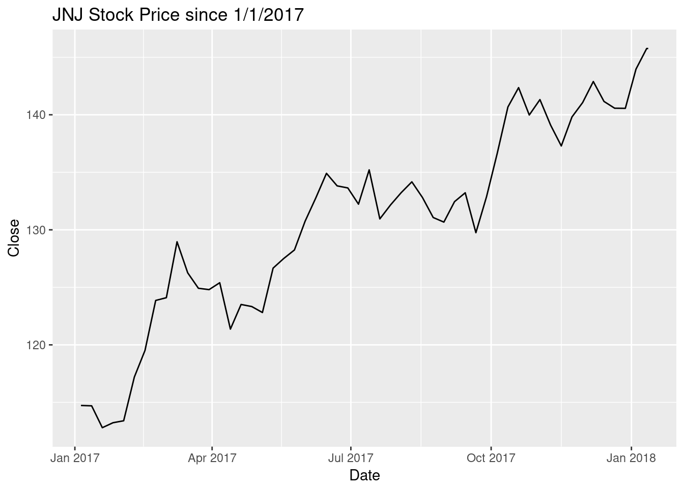
Single Random Walk
First, we’ll build a single random walk. A Monte Carlo simulation will need lots of random walks, but if we can do one, lots should be easy.
Do simplify things, I’m going to add an “index” variable instead of working explicitly with dates.
jnj17$idx <- 1:length(jnj17$Close)
jnj17$type <- "Actual"
Now, let’s make a random walk to predict the next 25 weeks of stock closing values. We’ll assume that the prices should have normally distributed changes around the most recent price and that the standard deviation will be half the average of the weekly ranges over the last year(ish). This last bit is pretty arbitrary, we could use a standard deviation \(1\), or something else justified by economics.
n<- length(jnj17$Close)
rw <- jnj17$Close[n]+cumsum(rnorm(25, mean = 0, sd = 0.5*mean(jnj17$High - jnj17$Low)))

#build new data.frame
rwData <- data.frame(idx=(n+1):(n+25), Close=rw, type=rep("RW",25))

#table
library(knitr)
kable(rwData)| idx | Close | type |
|---|---|---|
| 56 | 144.5784 | RW |
| 57 | 146.2035 | RW |
| 58 | 144.7451 | RW |
| 59 | 142.6243 | RW |
| 60 | 141.8303 | RW |
| 61 | 142.1619 | RW |
| 62 | 140.6649 | RW |
| 63 | 141.3005 | RW |
| 64 | 142.0169 | RW |
| 65 | 142.9144 | RW |
| 66 | 144.5575 | RW |
| 67 | 145.5519 | RW |
| 68 | 148.1797 | RW |
| 69 | 146.6338 | RW |
| 70 | 147.9975 | RW |
| 71 | 147.0684 | RW |
| 72 | 147.9050 | RW |
| 73 | 146.7997 | RW |
| 74 | 145.7820 | RW |
| 75 | 145.8861 | RW |
| 76 | 147.7343 | RW |
| 77 | 146.6477 | RW |
| 78 | 149.7615 | RW |
| 79 | 149.4796 | RW |
| 80 | 146.7478 | RW |
#plot
rbind.data.frame(select(jnj17, idx,Close,type), rwData) %>%
  ggplot(aes(x=idx,y=Close, col=type))+geom_line()+
  ggtitle("JNJ Actual and Predicted Price")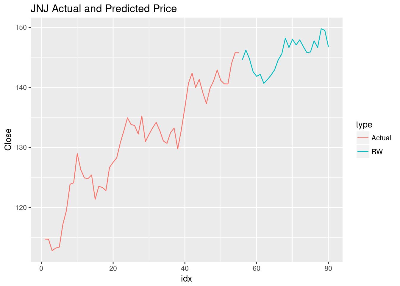
This is likely a bad prediction at any given index. The hope is that lots of similarly constructed predictions will give insight into the probability distribution of the future JNJ stock prices. This means we’ll need lots of random walks.
Multiple Random Walks
We just need to replicate what we did previously for an arbitrary number of times. To automate this, we’ll make a function to give a data frame with our random walk data, this will work with any similarly structured data (other stock data from Yahoo finance).
randWalk <- function(typeName, len, obsData){
    n<- length(obsData$Close)
    rw <- obsData$Close[n]+cumsum(rnorm(len, mean = 0, sd = 0.5*mean(obsData$High - obsData$Low)))

    #build new data.frame
    rwData <- data.frame(idx=(n+1):(n+len), Close=rw, type = rep(typeName,len))
    return(rwData)
}

#doing 7 random walks because of the colorblind palette
rwList <- lapply(1:7, function(x) {randWalk(paste("RW",x,sep=""),25,jnj17)})

rwDF <- as.data.frame(bind_rows(rwList))
jnjPred <- rbind.data.frame(select(jnj17,idx,Close,type), rwDF)

#store colorblind palette
cbbPalette <- c("#000000", "#E69F00", "#56B4E9", "#009E73", "#F0E442", "#0072B2", "#D55E00", "#CC79A7")

ggplot(jnjPred, aes(x=idx,y=Close,col=type)) +
  geom_line() + ggtitle("JNJ Predictions with Multiple Random Walks") +
  scale_color_manual(values=cbbPalette)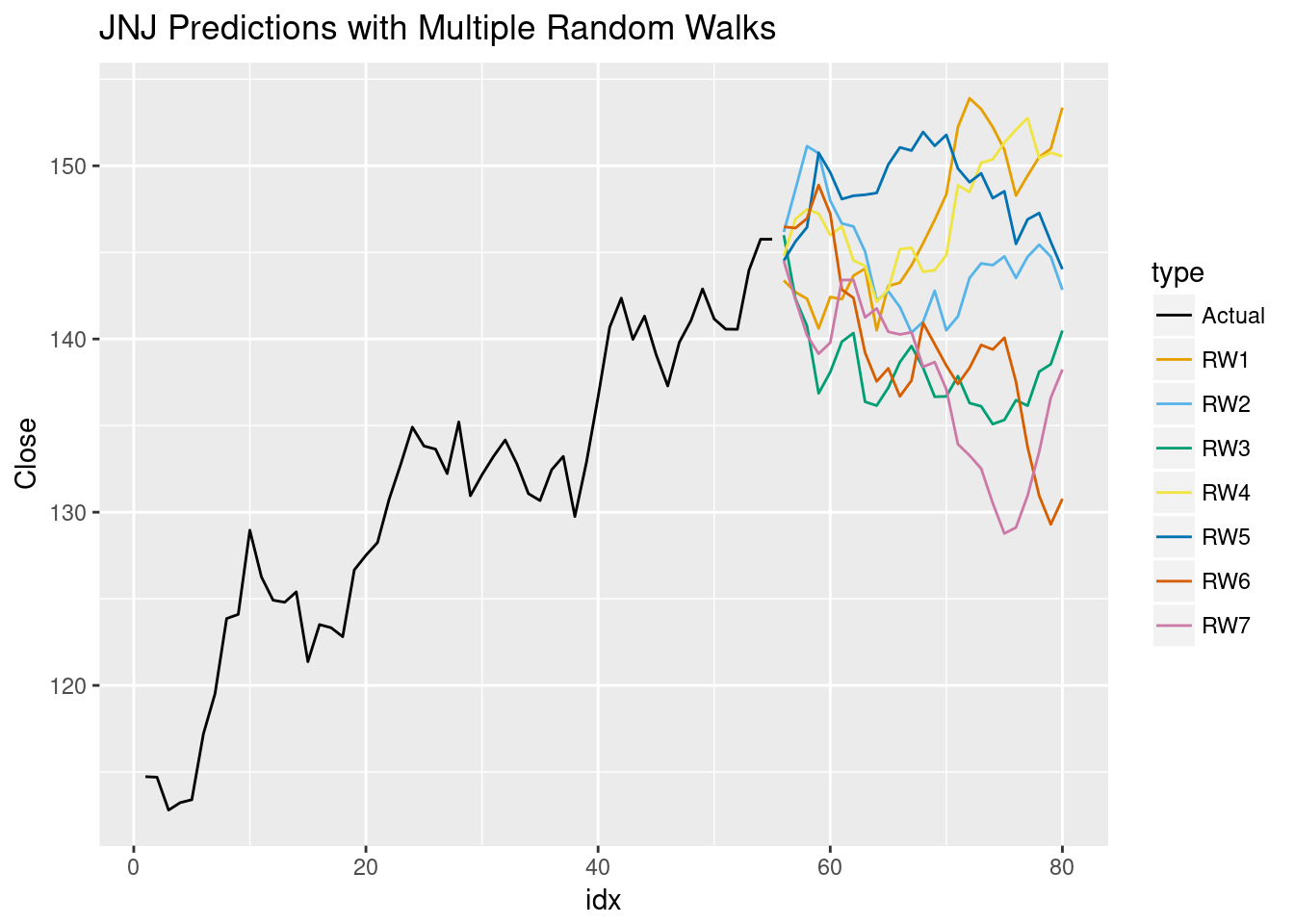
The collection of random walks are a random sample of all JNJ stock price predictions for the next 25 weeks. Because of how we build our predictions, we clearly see oscilation about the most recent actual close. By using a more informative prediction process, we may see more informative predictions but this would just alter our randWalk function. We can use this to clean up the graph a bit, we can plot the mean of the random walks and their range at each index.
rwDFreduced <- group_by(rwDF, idx) %>%
  summarise(meanPred=mean(Close), high = max(Close), low=min(Close)) %>%
  mutate(Close = meanPred, type="Prediction")

ggplot(jnj17, aes(x=idx,y=Close,col=type)) + geom_line() +
  geom_ribbon(data=rwDFreduced, aes(x=idx,ymin=low,ymax=high), fill="grey70", inherit.aes = FALSE) +
  geom_line(data=rwDFreduced, aes(x=idx,y=Close, col=type)) +
  ggtitle("JNJ 7 Random Walks Prediction Ribbon")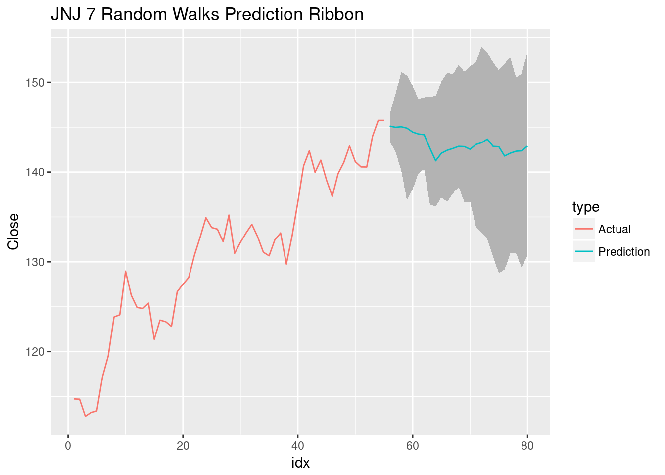
Due to the lack of any economic theory, I wouldn’t put much weight in this prediction but it would be easy to incorporate that into the random walk and the Monte Carlo simulation won’t change. Additionally, each time this code is re-run, the above ribbon can change noticeably.
With the ribbon, there’s no need to limit ourselves to 7 random walks. Let’s do more for a real Monte Carlo simulation (and maybe a better, or at least more stable, prediction).
rwList <- lapply(1:100, function(x) {randWalk(paste("RW",x,sep=""),25,jnj17)})
rwDF <- as.data.frame(bind_rows(rwList))
rwDFreduced <- group_by(rwDF, idx) %>%
summarise(meanPred=mean(Close), high = max(Close), low=min(Close)) %>%
mutate(Close = meanPred, type="Prediction")
ggplot(jnj17, aes(x=idx,y=Close,col=type)) + geom_line() +
geom_ribbon(data=rwDFreduced, aes(x=idx,ymin=low,ymax=high), fill="grey70", inherit.aes = FALSE) +
geom_line(data=rwDFreduced, aes(x=idx,y=Close, col=type)) +
ggtitle("JNJ 100 Random Walks Prediction Ribbon")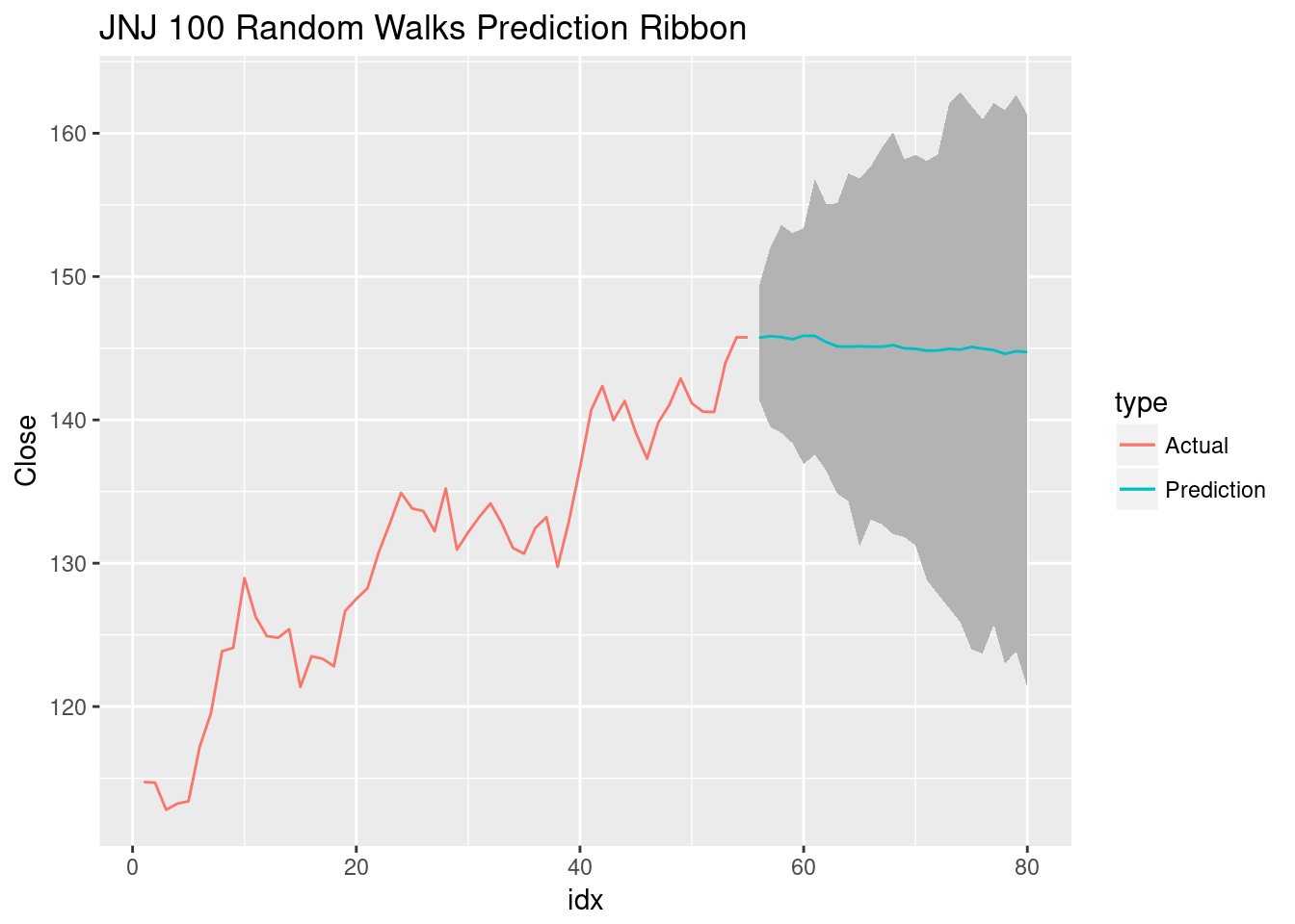 With so many random walks, it’s no surprise the prediction line (the mean of the random walks) is nearly flat, this is the Central Limit Theorem in action.