Edit 7/27/2018 I realized that MFL’s name change to WLC didn’t change the prefix of their courses, this broke my scrapper. Below is an updated post that deals with this.
Back in early May, I wrote a post about scraping the College of Idaho catalog: Counting Classes. Below if the same post (boring…) except that the “current catalog” has been updated. This is really a demonstration of reproducibility, the upstream data has changed and ideally all my code still works.
There are however, some problems - look at the old post and try to guess. If you guessed the hard-coded indices of
subjectText <- subjectText[79:122]
#keep url for each subject also
sub_url <- html_attr(subjectLinks, 'href')[79:122]
you’re right! The link positions on the page changed slightly, partly because of MFL changing their department name to WLC. However, they didn’t change the prefixes of the courses, so I’ll need to change the get_class_links function. The change required regular expressions, which I’m growing to love because of how clean they are with stringr it helps me overcome the PERL nightmares of my youth.
Begin Updated Original
At the College of Idaho, there’s been discussion about visualizing the curriculum as well as understanding the curriculum. Naturally this interests me as a chance to wallow in some complicated data (students are required to complete a major and 3 minors across 4 “peaks” rather than complete courses from a traditional “core”). I thought using R and a Neo4j graph database would be useful (something to look forward to) - but first I needed to get data from the catalogue!
Web Scraping
Web scraping is one the essential data science skills that I’m not as fluent in as I would like to be, so getting the course data from the catalogue is a nice chance to hone my skills. The rvest package (from Hadley Wickham) is a great tool for web scraping in R and combines well with stringr text manipulation functions and the SelectorGadget chrome extension.
We’ll start by getting a list of all subjects in the catalogue, with links to the subject page which has the class list in that subject.
base_url <- "http://collegeofidaho.smartcatalogiq.com"
base_url_ext <- "/en/current/Undergraduate-Catalog/Courses"

#read base page
base_html <- read_html(paste0(base_url,base_url_ext))
#extract links from base page
subjectLinks <- html_nodes(base_html, 'a')
#convert links to text
subjectText <- html_text(subjectLinks)
subjectText <- subjectText[79:122]
#keep url for each subject also
sub_url <- html_attr(subjectLinks, 'href')[79:122]

subDF <- str_split(subjectText,pattern= '-', n=2,
                   simplify=TRUE) %>% as.data.frame()
names(subDF) <- c("sub", "subject")
subDF <-mutate(subDF, sub = str_trim(sub, side = "both"),
               subject = str_trim(subject, side = "both"),
               url=paste0(base_url,sub_url))

kable(head(subDF),"html") %>%
kable_styling( bootstrap_options = c("striped", "hover", "condensed", "responsive"), full_width=FALSE) The kable_styling function is from the kableExtra package and provides some nice features to control kable style. Now we need to follow the link for each subject and get a dataframe of course numbers, names and urls for description, credit, and prerequisite info. The nice way of doing this is use purrr’s map_dfr function which is a more user friendly version of *apply and rbind.data.frame. As with apply, we’ll need a function to call on each subject.
get_class_list <- function(i){
  #get list of links on subject page
  class_links <- html_nodes(read_html(subDF$url[i]), 'a')
  #turn links to text
  class_list <- html_text(class_links)
  class_url <- html_attr(class_links, 'href')
  classDF <- data.frame(list=class_list, url=class_url)

  #only keep links for classes, each subject has
  #classes starting in a different position
  classDF <- classDF %>% filter(str_detect(list,
                                  "[:upper:]{2,3}-"))

    #We'll split on 1st space, discard everything after it and use
  #what's before it to build the required DF
  classDF <- separate(classDF, list,
                  into=c("id", "name"), sep = " ", extra = "merge")

  #two theater classes have typos -THE-###
  #this is solely dealing with that
  classDF$id <- str_replace(classDF$id, "-THE", "THE")

  #back to normal
  classDF <- separate(classDF, id, into =
                        c("sub", "number"), sep="-")

  #the id field has the last part of the new url, we need the
  #subject url with the course level (100,200,etc) then id
  classDF <- mutate(classDF, url=paste0(base_url,url))

  #several class names have '\n' in them, let's remove that now
  classDF <- mutate(classDF, name=str_replace_all(name, '\n',' '))

  return(classDF)
}

classes <- map_dfr(1:length(subDF$sub), get_class_list)
#add level variable (100,200, etc.)
classes <- classes %>% mutate(level=paste0(
          str_extract(number, '[:digit:]'),"00"))

kable(head(classes),"html") %>%
  kable_styling( bootstrap_options =
               c("striped", "hover", "condensed",
"responsive"), full_width=FALSE) | sub | number | name | url | level |
|---|---|---|---|---|
| ACC | 221 | Financial Accounting | http://collegeofidaho.smartcatalogiq.com/en/current/Undergraduate-Catalog/Courses/ACC-Accounting/200/ACC-221 | 200 |
| ACC | 222 | Managerial Accounting | http://collegeofidaho.smartcatalogiq.com/en/current/Undergraduate-Catalog/Courses/ACC-Accounting/200/ACC-222 | 200 |
| ACC | 318 | Intermediate Accounting I | http://collegeofidaho.smartcatalogiq.com/en/current/Undergraduate-Catalog/Courses/ACC-Accounting/300/ACC-318 | 300 |
| ACC | 320 | Intermediate Accounting II | http://collegeofidaho.smartcatalogiq.com/en/current/Undergraduate-Catalog/Courses/ACC-Accounting/300/ACC-320 | 300 |
| ACC | 323 | Electronic Accounting & Analysis | http://collegeofidaho.smartcatalogiq.com/en/current/Undergraduate-Catalog/Courses/ACC-Accounting/300/ACC-323 | 300 |
| ACC | 323 | Electronic Accounting & Analysis | http://collegeofidaho.smartcatalogiq.com/en/current/Undergraduate-Catalog/Courses/ACC-Accounting/300/ACC-323 | 300 |
Now we have the basic class info, on to some descriptive analysis.
The Counts
I should mention that this data is all from the current (2017-2018) catalogue, so it doesn’t reflect courses added, removed, or changed during this academic year. The most basic question is how many classes does CofI offer? Well, the 44 subjects offer 1026 courses, but how are they distributed across subject and level?
First, let’s group by subject to see which subjects offer the most and least courses.
group_by(classes, sub) %>%
  summarise(Count = n()) %>%
  arrange(desc(Count)) %>% head() %>%
  kable("html", caption =
          "Subjects with the Most Courses") %>%
  kable_styling( bootstrap_options = c("striped",
"hover", "condensed", "responsive"), full_width=FALSE) | sub | Count |
|---|---|
| HIS | 95 |
| BIO | 92 |
| ENG | 62 |
| MUS | 56 |
| POE | 51 |
| THE | 46 |
group_by(classes, sub) %>% summarise(Count = n()) %>%
  arrange(desc(Count)) %>% tail() %>%
  kable("html", caption = "Subjects with the Least Courses") %>%
  kable_styling( bootstrap_options = c("striped", "hover",
"condensed", "responsive"), full_width=FALSE) | sub | Count |
|---|---|
| ASN | 3 |
| EDUSPA | 3 |
| ECN | 2 |
| ESL | 2 |
| FYS | 2 |
| STS | 1 |
Clearly, History doesn’t teach all of those classes every semester. It would be interesting to incorporate frequency of classes into this analysis, but that requires data from elsewhere since CofI doesn’t typically put course frequency into the catalogue.
Second, we can ignore subjects and look at the distribution of courses at different levels:
group_by(classes, level) %>% summarise(Count = n()) %>%
  kable("html", caption = "Number of Courses at each Level") %>%
  kable_styling( bootstrap_options = c("striped", "hover",
"condensed", "responsive"), full_width=FALSE) | level | Count |
|---|---|
| 000 | 1 |
| 100 | 163 |
| 200 | 232 |
| 300 | 413 |
| 400 | 217 |
Finally, we can look at the distribution grouped by subject and level but because of the range of course counts at each subject, it’s probably better to work with proportions rather than counts. I’ll also order by decreasing proportion and note that if a subject (like accounting) doesn’t teach any classes of a particular level, we won’t see zeros in the list.
subCnt <- group_by(classes, sub) %>% summarise(Count_s = n())
sublevDF <- group_by(classes, sub, level) %>%
  summarise(Count_sl = n())

sublevDF <- inner_join(sublevDF, subCnt, by="sub") %>%
  mutate(sub.prop = round(Count_sl/Count_s, 4)) %>%
  dplyr::select(sub, level, sub.prop) %>%
  arrange(desc(sub.prop))

kable(sublevDF, "html", caption = "Proportion of Subject's
      Courses at each Level") %>%
  kable_styling( bootstrap_options = c("striped", "hover",
          "condensed", "responsive"), full_width=FALSE) %>%
scroll_box(width="100%", height = "250px")| sub | level | sub.prop |
|---|---|---|
| ECN | 200 | 1.0000 |
| EDUSPA | 100 | 1.0000 |
| ESL | 100 | 1.0000 |
| FYS | 100 | 1.0000 |
| STS | 100 | 1.0000 |
| ATHSOC | 400 | 0.8333 |
| HHPA | 100 | 0.8276 |
| ARH | 300 | 0.7500 |
| MFL | 400 | 0.7273 |
| HIS | 300 | 0.6737 |
| ASN | 300 | 0.6667 |
| IND | 300 | 0.6471 |
| HSC | 300 | 0.6000 |
| CHI | 100 | 0.5714 |
| GER | 200 | 0.5714 |
| BIO | 300 | 0.5652 |
| SPA | 300 | 0.5357 |
| ACC | 400 | 0.5333 |
| POE | 300 | 0.5294 |
| SOC | 300 | 0.5294 |
| PHI | 300 | 0.5263 |
| PHY | 200 | 0.5161 |
| EDU | 400 | 0.5000 |
| LAS | 400 | 0.5000 |
| LSP | 200 | 0.5000 |
| SPE | 300 | 0.5000 |
| ENV | 300 | 0.4762 |
| ENG | 300 | 0.4677 |
| CHE | 400 | 0.4474 |
| PSY | 300 | 0.4390 |
| BUS | 400 | 0.4186 |
| THE | 300 | 0.4130 |
| ENG | 200 | 0.4032 |
| CSC | 400 | 0.4000 |
| FRE | 200 | 0.4000 |
| JOURN | 400 | 0.4000 |
| MUSAP | 400 | 0.4000 |
| REL | 300 | 0.4000 |
| BUS | 300 | 0.3953 |
| HHP | 300 | 0.3864 |
| EDU | 300 | 0.3750 |
| GEO | 100 | 0.3750 |
| GEO | 400 | 0.3750 |
| REL | 200 | 0.3667 |
| MS | 200 | 0.3636 |
| ART | 200 | 0.3548 |
| ACC | 300 | 0.3333 |
| ASN | 400 | 0.3333 |
| HHP | 400 | 0.3182 |
| CHE | 300 | 0.3158 |
| THE | 200 | 0.3043 |
| MUS | 100 | 0.3036 |
| FRE | 100 | 0.3000 |
| FRE | 300 | 0.3000 |
| JOURN | 200 | 0.3000 |
| JOURN | 300 | 0.3000 |
| ATH | 200 | 0.2941 |
| ATH | 300 | 0.2941 |
| ART | 300 | 0.2903 |
| CHI | 200 | 0.2857 |
| GER | 300 | 0.2857 |
| MAT | 200 | 0.2857 |
| MS | 300 | 0.2727 |
| PSY | 400 | 0.2683 |
| CSC | 200 | 0.2667 |
| PHI | 200 | 0.2632 |
| MAT | 100 | 0.2571 |
| MAT | 400 | 0.2571 |
| ARH | 200 | 0.2500 |
| GEO | 300 | 0.2500 |
| LAS | 300 | 0.2500 |
| LSP | 400 | 0.2500 |
| MUS | 200 | 0.2500 |
| MUS | 300 | 0.2500 |
| SPE | 100 | 0.2500 |
| SPE | 200 | 0.2500 |
| ATH | 400 | 0.2353 |
| CSC | 100 | 0.2000 |
| HSC | 100 | 0.2000 |
| HSC | 400 | 0.2000 |
| MAT | 300 | 0.2000 |
| MUSAP | 100 | 0.2000 |
| MUSAP | 200 | 0.2000 |
| MUSAP | 300 | 0.2000 |
| BIO | 100 | 0.1957 |
| PSY | 200 | 0.1951 |
| ART | 400 | 0.1935 |
| PHY | 400 | 0.1935 |
| ENV | 200 | 0.1905 |
| ENV | 400 | 0.1905 |
| MFL | 200 | 0.1818 |
| MS | 100 | 0.1818 |
| MS | 400 | 0.1818 |
| MUS | 400 | 0.1786 |
| SPA | 200 | 0.1786 |
| SPA | 400 | 0.1786 |
| ATH | 100 | 0.1765 |
| IND | 200 | 0.1765 |
| POE | 100 | 0.1765 |
| POE | 200 | 0.1765 |
| SOC | 200 | 0.1765 |
| SOC | 400 | 0.1765 |
| THE | 400 | 0.1739 |
| ATHSOC | 200 | 0.1667 |
| ART | 100 | 0.1613 |
| PHY | 100 | 0.1613 |
| HHP | 200 | 0.1591 |
| PHI | 400 | 0.1579 |
| BIO | 200 | 0.1522 |
| HIS | 200 | 0.1474 |
| CHI | 400 | 0.1429 |
| ENV | 100 | 0.1429 |
| GER | 400 | 0.1429 |
| HHPA | 200 | 0.1379 |
| HIS | 400 | 0.1368 |
| HHP | 100 | 0.1364 |
| ACC | 200 | 0.1333 |
| CSC | 300 | 0.1333 |
| REL | 400 | 0.1333 |
| CHE | 100 | 0.1316 |
| PHY | 300 | 0.1290 |
| EDU | 200 | 0.1250 |
| LAS | 100 | 0.1250 |
| LAS | 200 | 0.1250 |
| LSP | 100 | 0.1250 |
| LSP | 300 | 0.1250 |
| IND | 100 | 0.1176 |
| POE | 400 | 0.1176 |
| SOC | 100 | 0.1176 |
| ENG | 400 | 0.1129 |
| THE | 100 | 0.1087 |
| SPA | 100 | 0.1071 |
| CHE | 200 | 0.1053 |
| REL | 100 | 0.1000 |
| PSY | 100 | 0.0976 |
| BUS | 100 | 0.0930 |
| BUS | 200 | 0.0930 |
| MFL | 300 | 0.0909 |
| BIO | 400 | 0.0870 |
| IND | 400 | 0.0588 |
| PHI | 100 | 0.0526 |
| HIS | 100 | 0.0421 |
| HHPA | 300 | 0.0345 |
| MUS | 000 | 0.0179 |
| ENG | 100 | 0.0161 |
Course Name Word Cloud
Now for a different type of counting, let’s make a word cloud of words in course names. I would rather use the wordcloud2 package which allows for some interesting visualizations, but it relies on javascript which doesn’t play well with a static site generator (but a shiny app would work). We’ll need to load some additional packages and split up the name data into words and frequencies, after doing a little cleaning of the names.
library(devtools)
library(tm)
library(SnowballC)
library(wordcloud)

#Load and clean
wordFreq <- Corpus(VectorSource(classes$name))
wordFreq <- tm_map(wordFreq, PlainTextDocument)
wordFreq <- tm_map(wordFreq, content_transformer(tolower))
wordFreq <- tm_map(wordFreq, removePunctuation)
wordFreq <- tm_map(wordFreq, removeWords, c("a", "the", "and", "for"))
wordFreq <- tm_map(wordFreq, stripWhitespace)

#build TDM and DF of words and frequencies
wordTDM <- TermDocumentMatrix(wordFreq)
wordTDM<- wordTDM %>% as.matrix() %>% rowSums() %>% sort()
wordDF <- data.frame(word=names(wordTDM), freq=wordTDM)

pal <- brewer.pal(9, "Purples")[-(1:3)]

wordcloud(words=wordDF$word, freq=wordDF$freq,
          min.freq = 6,  random.order = FALSE, rot.per = .25,
          scale = c(3,.5), colors = pal)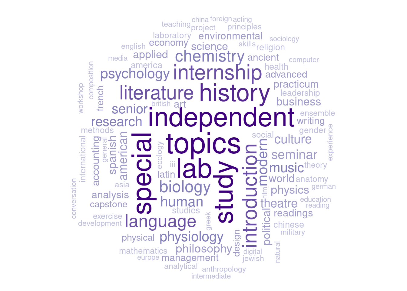
The special topics and independent study classes that almost all subjects have along with lab and introduction are not too surprising. History, with it’s high course count and the fact that it appears in other subjects (History of Math or Music History) is also not surprising. Beyond that, the wordcloud shows a nice diversity of disciplines and unifying ideas.
Clearly this is just scratching the surface of exploring a college’s curriculum and it would be interesting to compare similar schools in addition to exploring deeper into course descriptions and the links formed by prerequisites and major/minor requirements.