Update 7/23/2019 Various package updates have created problems with showing more than one javascript plot on a post. I’ve added calls to htlwidgets::onRender to get at least one plot displayed. I may revisit this, but the interaction between hugo, blogdown, and various javascript libraries (chorddiag, networkD3, D3, data tables, etc) is more than I’m able to dive into at the moment.
This post is about a type of visualization the will hopefully help see how students “flow” through college. The data is an anonymized selection of Math and Math-Computer Science majors at the College of Idaho, and for simplicity we’ll only be using the math and computer science courses. Out goal is to produce the following Sankey Diagram, which is really just a graph (in the discrete math sense - nodes connected by edges) where the edges are scaled by weight, in this case the number of students taking course A then B will be reflected in the width of the link between A and B. The sankeyNetwork command also adjust the node layout to minimize edge crossing and have a general “left to right” aspect.
sn <- sankeyNetwork(Links = edgeDFTemp, Nodes = nodeDFTemp, Source = "source",
              Target = "target", Value = "value", NodeID = "id",
              nodeWidth = 20, fontSize = 8, units = "students")

htmlwidgets::onRender(sn, 'document.getElementsByTagName("svg")[0].setAttribute("viewBox", "")')
The Data
Following general practice, let’s first look at the data that we’ll be using. I’ve said this is some anonymized student data consisting of an id (hashed, not actual student id’s), a course prefix and number crs, and a standardized year value std.year. This std.year variable indicates when a student is taking the course during their “college career” with 0.0 meaning first fall semester, 1.4 meaning spring of their second year. The first digit is basically the number of years of college completed (\(0,1,2,\) or \(3\)) and the second codes the semester type (\(0\) is fall, \(2\) is winter, \(4\) is spring and \(6\) is summer). These are numeric so I could do arithmetic and standardize things. The point is to help us see students taking a course like CSC-150 (Intro to CS) in their freshman versus junior years, how they got there, and what they do next.
Now that you understand the variables, here’s a glimpse of the data (and the packages I need for the post):
library(dplyr)
library(ggplot2)
library(stringr)
library(tidyr)
library(DT)
library(networkD3)

students <- read.csv("../../static/files/math-major-anon.csv", header=TRUE)
students %>% head() %>% knitr::kable()| id | crs | std.year |
|---|---|---|
| 8b551f6ba68aef2c9da1bf682e44716c | CSC-150 | 0.4 |
| 8b551f6ba68aef2c9da1bf682e44716c | MAT-252 | 0.4 |
| 8b551f6ba68aef2c9da1bf682e44716c | MAT-175 | 0.0 |
| 5069338819f368fb8960772475069d02 | CSC-150 | 0.4 |
| 5069338819f368fb8960772475069d02 | MAT-175 | 0.4 |
| 5069338819f368fb8960772475069d02 | MAT-150 | 0.0 |
Let’s also explore the data a little. Here’s the distribution of std.year’s:
ggplot(students, aes(x=as.factor(std.year)))+geom_bar()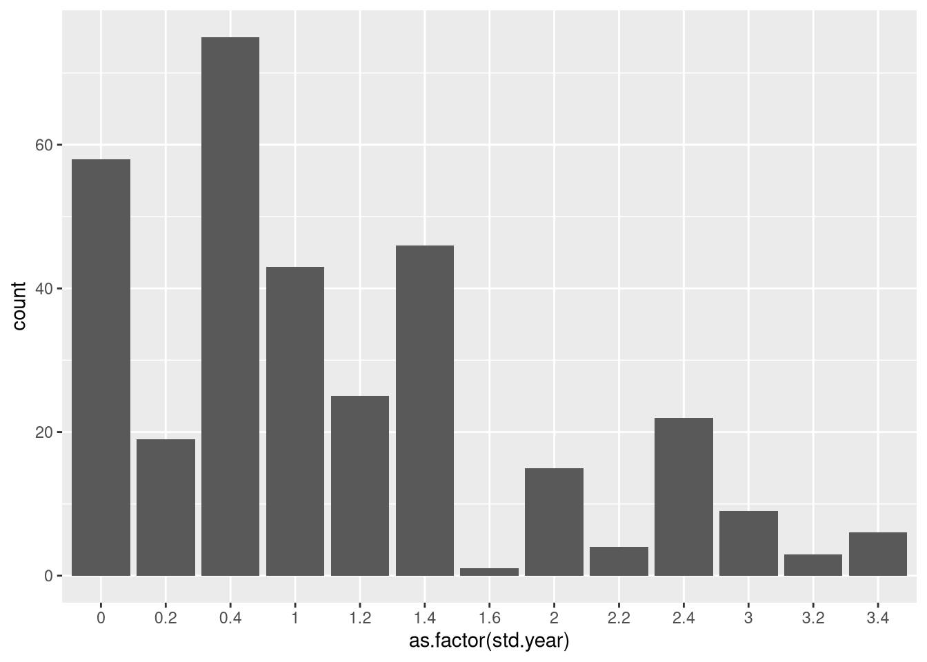
Clearly, most students are early in college and few students take summer math or CS courses (we don’t offer them, except internships and occasionally intro. stats).
Next, we’ll look at the courses by popularity (within our dataset):
library(widgetframe)

students %>% group_by(crs) %>%
  summarise(Count = n_distinct(std.year),
            Num.Students = n_distinct(id)) %>%
  arrange(desc(Num.Students), desc(Count)) %>%
  datatable() %>%
  frameWidget(height = 550, width = "100%")
Since these are math and math/cs majors, it’s not surprising that single variable calculus and intro cs are the two most common courses (they’re required of all students in this dataset). What may be more interesting is that students have completed single variable calculus (MAT-175) at 4 different points in their trajectory towards a math or math/cs major. This means that we will expect 4 nodes for MAT-175 in our sankey diagram (this may get messy).
There is one thing we can do to make things a little cleaner. The MAT-28x intro to proofs courses should be combined since students usually only take MAT-280, MAT-281, MAT-282, etc. depending on what’s offered the year they need to take it.
students$crs <- str_replace(students$crs, "MAT-28[:digit:]{1}", "MAT-28X")Building Nodes and Edges
The sankeyNetwork command, like most networkD3 commands, needs to be given a graph (nodes and edges). Unfortunately, it’s not smart enough to build it from our students data frame, we need to build it.
The nodes are easier, so we’ll start there. We want an id for each node that combines the crs and std.year variables, so I’ll keep those and make a new id column (note this will lose all student info).
nodes <- group_by(students, crs, std.year) %>%
  summarise(cnt = n()) %>% ungroup() %>%
  select(name=crs, std.year) %>%
  unite(id, name, std.year, sep="_", remove=FALSE)

nodes %>% head() %>% knitr::kable()| id | name | std.year |
|---|---|---|
| CSC-150_0 | CSC-150 | 0.0 |
| CSC-150_0.4 | CSC-150 | 0.4 |
| CSC-150_1 | CSC-150 | 1.0 |
| CSC-150_1.4 | CSC-150 | 1.4 |
| CSC-150_2.4 | CSC-150 | 2.4 |
| CSC-150_3 | CSC-150 | 3.0 |
The group_by, summarise, and ungroup sequence is just a way to collapse down to each distinct crs, std.year pair that occurs in the data. We now have 89 nodes that will appear in the diagram.
Now for the edges. We’re going to create a data frame of “source” nodes and another of “target” nodes (remember we’re building a directed graph). A full join of the two will give all possible edges, so we’ll then remove those that aren’t needed. Most of the extra edges will be those connecting what a student did during fall of freshmen year to all subsequent courses, not just the immediate “next” course that we want plotted. These seem far easier to remove then to selectively build a much more careful join (only joining pairs with “adjacent” standard years).
Here’s the code to build the first pass of an edge list data frame:
#build source data
s.crs <- select(students, s.name=crs, s.std.year=std.year, id)
s.crs <- s.crs[!duplicated(s.crs),]
#build target data
t.crs <- select(students, t.name=crs, t.std.year=std.year, id)
t.crs <- t.crs[!duplicated(t.crs),]
#join and remove self-loops and backward edges
edgePerStudent <- full_join(s.crs, t.crs) %>%
  filter(s.name!=t.name, s.std.year<t.std.year) %>%
  arrange(id, s.std.year, t.std.year)

edgePerStudent %>% head() %>% knitr::kable()| s.name | s.std.year | id | t.name | t.std.year |
|---|---|---|---|---|
| CSC-150 | 0.4 | 09d4fb320db773a123eb97e7260caba1 | MAT-275 | 1.0 |
| MAT-175 | 0.4 | 09d4fb320db773a123eb97e7260caba1 | MAT-275 | 1.0 |
| CSC-150 | 0.4 | 09d4fb320db773a123eb97e7260caba1 | MAT-28X | 1.2 |
| MAT-175 | 0.4 | 09d4fb320db773a123eb97e7260caba1 | MAT-28X | 1.2 |
| CSC-150 | 0.4 | 09d4fb320db773a123eb97e7260caba1 | MAT-352 | 1.4 |
| MAT-175 | 0.4 | 09d4fb320db773a123eb97e7260caba1 | MAT-352 | 1.4 |
As the name implies, we now have a data frame where each row is an edge from a distinct student. It’s important to note that I’ve arranged this in order for what comes next: id, then source standard year, and then target standard year. This data frame has 1112 rows, which is too many. We have extra edges formed by paths of what we want to keep and we need to collapse to have an edge with a weight equal to number of students taking that sequence of courses. The second part is easy (we could do a group_by and summarise now, but we would over count). The first part is possibly the ugliest R code I’ve written in a while, but it works and without messy lags and functional trickery is fairly straightforward. I initially tried to use a “run-length encoding”, but the resulting objects became to cumbersome (an rle object isn’t a data frame or a list or anything else “nice”), so here’s a for loop in R:
#build edges
edgeDF <- edgePerStudent[1,] #got to start somewhere
for(i in 2:nrow(edgePerStudent)){
  if(edgeDF[nrow(edgeDF),]$id != edgePerStudent[i,]$id){
    #different id's count
    edgeDF <- rbind.data.frame(edgeDF, edgePerStudent[i,])
  }
  else if(edgeDF[nrow(edgeDF),]$s.std.year == edgePerStudent[i,]$s.std.year & edgeDF[nrow(edgeDF),]$t.std.year == edgePerStudent[i,]$t.std.year){
    #same source and target as counting counts
    edgeDF <- rbind.data.frame(edgeDF, edgePerStudent[i,])
  }
  else if(edgeDF[nrow(edgeDF),]$t.std.year == edgePerStudent[i,]$s.std.year){
    #if last counted target is current source, it counts
    edgeDF <- rbind.data.frame(edgeDF, edgePerStudent[i,])
  }

}

#now count edge weights
edgeDF <- group_by(edgeDF, s.name, s.std.year, t.name,t.std.year) %>%
  summarise(value=n_distinct(id))
edgeDF <- unite(edgeDF, s.id, s.name,s.std.year, sep="_", remove=FALSE) %>%
  unite(t.id, t.name,t.std.year, sep="_", remove = FALSE)

edgeDF %>% head() %>% knitr::kable()| s.id | s.name | s.std.year | t.id | t.name | t.std.year | value |
|---|---|---|---|---|---|---|
| CSC-150_0 | CSC-150 | 0.0 | CSC-160_0.4 | CSC-160 | 0.4 | 1 |
| CSC-150_0 | CSC-150 | 0.0 | MAT-175_0.4 | MAT-175 | 0.4 | 1 |
| CSC-150_0 | CSC-150 | 0.0 | MAT-212_0.2 | MAT-212 | 0.2 | 1 |
| CSC-150_0 | CSC-150 | 0.0 | MAT-28X_0.2 | MAT-28X | 0.2 | 3 |
| CSC-150_0.4 | CSC-150 | 0.4 | CSC-152_1 | CSC-152 | 1.0 | 8 |
| CSC-150_0.4 | CSC-150 | 0.4 | MAT-175_1 | MAT-175 | 1.0 | 3 |
Now we have 198 edges, with the desired weights for the sankey diagram.
Making the Diagram
Now we just call sankeyNetwork and we’re done right? No, because we have data in R that we have to send to JavaScript to do the plotting so there’s a little book-keeping left to do. First, we need numeric node id’s and we need those id’s in the edge data.
#replace character s.id and t.id with numbers
nodes$node.id <- 1:nrow(nodes)
edgeDF <- inner_join(edgeDF, nodes, by=c("s.id"="id"))
edgeDF <- select(edgeDF, -s.id, source=node.id)
edgeDF <- inner_join(edgeDF, nodes, by=c("t.id"="id"))
edgeDF <- select(edgeDF, -t.id, target=node.id)
Next is the big conflict between R and almost every other programming language: indexing. R starts counting at 1, but JavaScript starts at 0 (as does Python, C/C++, Java, …) so we’ll have to re-index our node id’s. I’ll also replace everything after the first digit of std.year info in the node id variable, with a string indicating the semester.
#switch to zero indexing for javascript
edgeDFTemp <- mutate(edgeDF, source=source-1, target = target-1)
nodeDFTemp <- mutate(nodes, nid = node.id-1, id =
                       ifelse(str_detect(id, "\\.6"),
                              str_replace(id, "\\.6","SU"),
                              ifelse(str_detect(id, "\\.4"),
                                     str_replace(id, "\\.4", "SP"),
                                     ifelse(str_detect(id, "\\.2"),
                                            str_replace(id, "\\.2", "W"),
                                            str_c(id, "FA")))))

sn2 <- sankeyNetwork(Links = edgeDFTemp, Nodes = nodeDFTemp, Source = "source",
              Target = "target", Value = "value", NodeID = "id",
              nodeWidth = 20, fontSize = 8, units = "students")
htmlwidgets::onRender(sn2, 'document.getElementsByTagName("svg")[2].setAttribute("viewBox", "")')