The Basic Idea

Like any iterative algorithm, the big picture behind the EM algorithm is to converge to values given some initial guess. For our purposes, we want to converge to the parameters of a Gaussian mixture model given observed data, a number of Gaussians being mixed, and guesses for the initial means and standard deviations of the mixture components. This is one of the major practical uses of the EM algorithm: determining unknown parameters of mixture model components.

The algorithm repeats two key steps: Expectation and Maximization. The expectation step calculates probabilities of each data-point being in a mixture component. The maximization step uses these probabilities to update (a) means and standard deviations of mixture components and (b) the proportion of data-points in each component. There’s not much here that’s special to the case of Gaussian mixture models (GMM’s), except where we use normal distributions and the parameters we compute in the maximization step.

Note: The following functions are intended to be easy to understand as opposed to highly optimized with great error handling. If you’re estimating components of a Gaussian Mixture model in a production environment, Scikit-Learn has excellent clustering routines that will be far more robust and efficient than anything here.

import numpy as np
import pandas as pd
import matplotlib.pyplot as plt
import seaborn as sns
import scipy
from scipy.stats import norm
def expectation_probabilities_gmm(data, mean_vect, sd_vect, fracPerComp):
    ret_probs = np.zeros([len(data),len(mean_vect)])
    for i in range(len(data)):
        for j in range(len(mean_vect)):
            ret_probs[i,j] = (fracPerComp[j]*norm.pdf(data[i],mean_vect[j],sd_vect[j]))
        ret_probs[i,:] = ret_probs[i,:]/np.sum(ret_probs[i,:])
    return(ret_probs)

def maximization_params_gmm(expect_probs, data):
    clust_weights = [np.sum(expect_probs[:,j]) for j in
        range(np.shape(expect_probs)[1])]
    new_means = np.divide([np.sum(expect_probs[:,j]*data[:]) for
        j in range(np.shape(expect_probs)[1])],clust_weights)
    new_sds = np.divide([np.sum(expect_probs[:,j]*(data[:]-new_means[j])*(data[:]-new_means[j])) for j in range(np.shape(expect_probs)[1]) ], clust_weights)
    new_sds = np.sqrt(new_sds)
    new_frac = np.divide(clust_weights,np.shape(expect_probs)[0])
    return new_means, new_sds, new_frac;

def log_likelihood(data, mean_vect, sd_vect, fracPerComp):
  ret_probs = np.zeros([len(data),len(mean_vect)])
  for i in range(len(data)):
      for j in range(len(mean_vect)):
          ret_probs[i,j] = (fracPerComp[j]*norm.pdf(data[i],mean_vect[j],sd_vect[j]))
      row_sums = np.sum(ret_probs[i,:])
  loglike = np.sum(np.log(row_sums))
  return(loglike)

Observed Mixture Data

I don’t have a nice real-world GMM dataset, but we can easily manufacture some:

np.random.seed(seed=123987) #reproducibility
vals = [np.random.normal(5, .5, 100), np.random.normal(3, 1, 100), np.random.normal(6.5,1.25,100)]
grps = ['A','B','C']
#build dataframe
df = pd.concat([pd.DataFrame({"group":grps[i], "value":vals[i]}) for i in range(0,3)], axis=0, ignore_index=True)

Initially I had written this with 3 separate vectors of values and 3 data-frames that I then glued together. Then I remembered one of my favorite things about python: list comprehensions! Clearly I’ve made heavy use of them in the above functions as well.

With the group column in our dataframe, we can easily see the three components of the mixture:

#grouped
plt.figure(figsize=(3,3))
plots = sns.FacetGrid(data=df, hue="group", legend_out=True)
plots.map(sns.distplot,'value', kde_kws={"shade":False},rug_kws={"alpha":.3}, rug=True, kde=True, hist=False)
plt.show()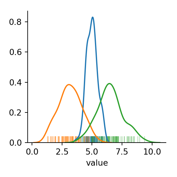

In practice though, we would only be able to see the full distribution of our data:

plt.close() #get a blank plot rather than overlay on our last distplots
plt.figure(figsize=(3,3))
sns.distplot(df['value'], rug=True, kde=True, hist=False)
plt.show()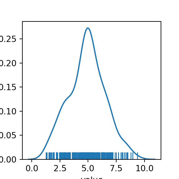

The “shoulders” on the curve given a hint that we may be dealing with an underlying mixture model of 3 components. But how “non-normal” is our data? We can run a Shapiro-Wilkes test and compare with the same number of points sampled from a single normal distribution to get an idea.

##Shapiro-Wilkes test
print(scipy.stats.shapiro(df['value']))

## (0.9909396767616272, 0.0613214448094368)

The second value in this tuple is the p-value associated to a null hypothesis that our data is from a single normal distribution. In this case we would fail to reject that our observed data is different from a sample from a single normal distribution at the customary \(0.05\) significance level. More evidence that p-values and significance tests can miss important details.

We can also compare to simulated data sampled from a true normal distribution with the same mean and standard deviation as our observed data to see how close our data is to being normal.

##compare with true normal sample
simDF = pd.DataFrame({"type":"simulated", "value":np.random.normal(df['value'].mean(), df['value'].std(), 300)})
simDF = pd.concat([pd.DataFrame({"type":"sample", "value":df['value']}), simDF], axis=0, ignore_index=True)
plt.figure(figsize=(3,3))
plotsim = sns.FacetGrid(data=simDF, hue="type")
plotsim.map(sns.distplot,'value', kde_kws={"shade":False},rug_kws={"alpha":.3}, rug=True, kde=True, hist=False)
plt.show()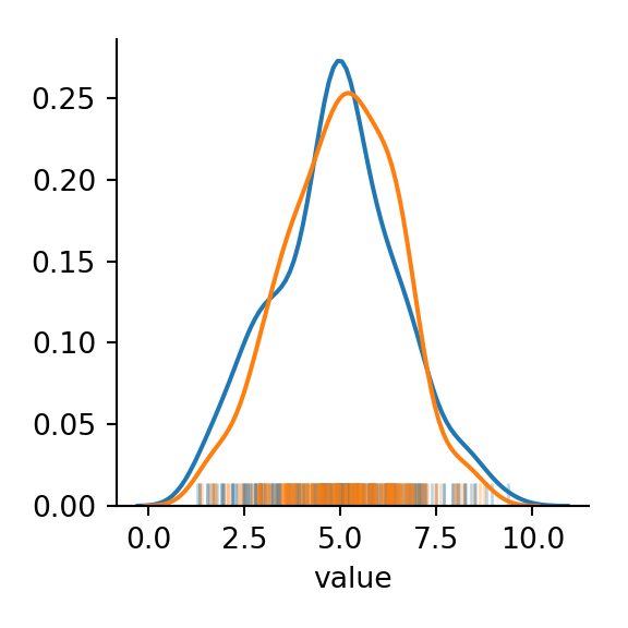

Running The EM

Here’s a function to handle calling the E and M steps and holding the results of each. This will be handle to look at how the process converges.

def run_em(data, init_means, init_sds, init_frac, num_iterations):
    ret_means = np.zeros((num_iterations,len(init_means)))
    ret_sds = np.zeros((num_iterations,len(init_means)))
    ret_fracs = np.zeros((num_iterations,len(init_means)))
    ret_ll = np.zeros(num_iterations)
    ret_means[0,:] = init_means
    ret_sds[0,:] = init_sds
    ret_fracs[0,:] = init_frac
    for i in range(num_iterations-1):
        ret_ll[i]=log_likelihood(data, ret_means[i,:],ret_sds[i,:], ret_fracs[i,:])
        new_probs = expectation_probabilities_gmm(data, ret_means[i,:],ret_sds[i,:], ret_fracs[i,:])
        ret_means[i+1,:], ret_sds[i+1,:],ret_fracs[i+1,:] = maximization_params_gmm(new_probs, data)
    return ret_means, ret_sds, ret_fracs, ret_ll;

Now we can make some guesses and run the EM algorithm. Based on the distribution of all the data, it looks like there are irregularities around 3, 5.5, and 7 - so those will be our means. We’ll assume variance of 1 and equal size for all groups.

means = [3,5.5, 7]
sds = [1,1,1]
fracs = [1/3,1/3,1/3]
mu,sigma,frac,ll = run_em(df['value'], means, sds, fracs, 50)

We can then easily use matplotlib to see how these change over the iterations:

plt.figure(figsize=(5,5))
plt.subplot(2,2,1)
plt.plot(mu)
plt.title("Means")
plt.xlabel("Iteration")
plt.xticks([10*(i+1) for i in range(5)])
plt.subplot(2,2,2)
plt.plot(sigma)
plt.title("Std. Deviations")
plt.xlabel("Iteration")
plt.xticks([10*(i+1) for i in range(5)])
plt.subplot(2,2,3)
plt.plot(frac)
plt.title("Fraction Per Cluster")
plt.xlabel("Iteration")
plt.xticks([10*(i+1) for i in range(5)])
plt.subplot(2,2,4)
plt.plot(ll[0:48]) #last ll value hasn't been calculated
plt.title("Log-Likelihood")
plt.xlabel("Iteration")
plt.xticks([10*(i+1) for i in range(5)])
plt.tight_layout()
plt.show()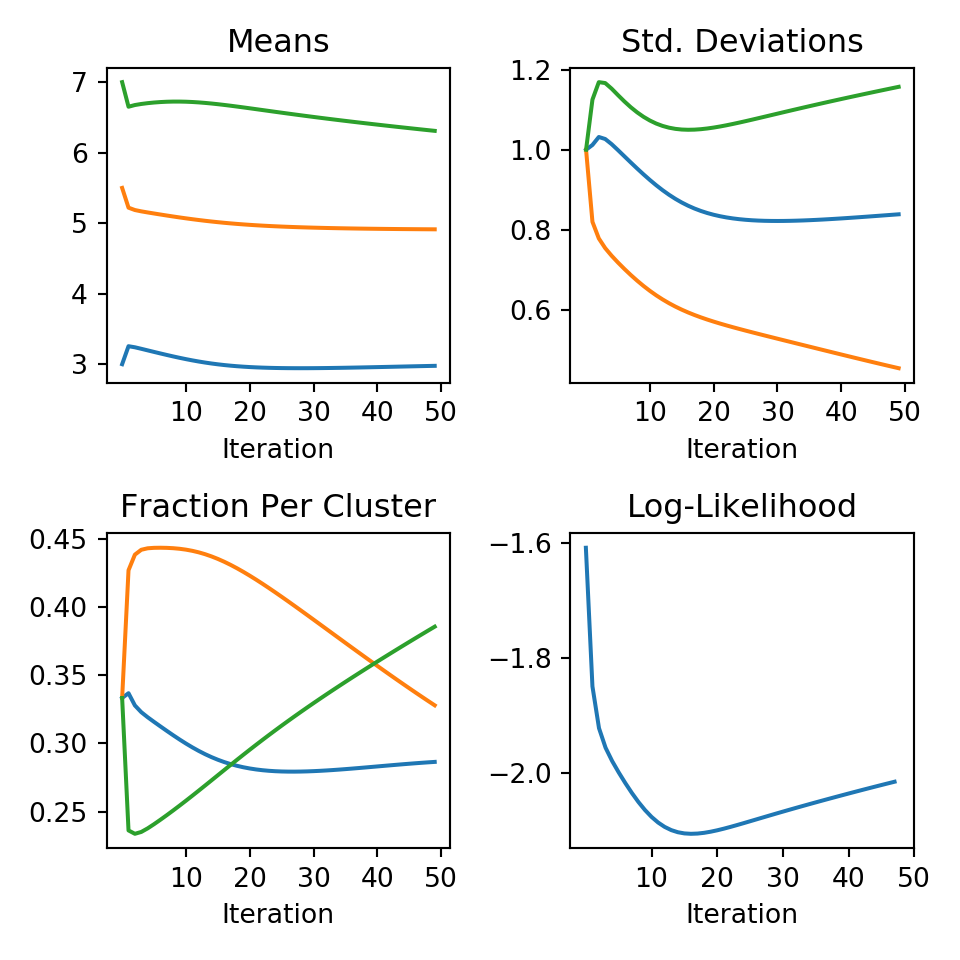

This looks like we had convergence fairly quickly, except the fraction of points per cluster - but our y-scale is very narrow. In the end our estimates are:

print("Means:", mu[49,:])

## Means: [2.9767655  4.91279169 6.30925586]

print("Std. Dev.:", sigma[49,:])

## Std. Dev.: [0.83852695 0.45363153 1.15733853]

print("Fraction per Cluster:", frac[49,:])

## Fraction per Cluster: [0.28652637 0.32794345 0.38553017]

Since our mixture components had means \(3, 5, 6.5\) and standard deviations \(1, 0.5, 1.25\) we did pretty good. The main difference is the points where the normal distributions overlap with “high” probability. This is where any clustering algorithm will break down. Despite how close our data was to a single normal distribution, the EM algorithm was able to divide the observations into 3 groups with means and standard deviations almost equal to the actual cluster parameters.

I want to show some visuals of our mean and std. dev. estimates with the data and how the clusters evolve, but this post has gotten a little long. Look forward to part 2 soon…