While continuing to work through BDA3, and decided to revisit some of the earlier exercises that I had done in R. Problem 9 of chapter 1 asks to simulate a medical clinic with 3 doctors, patients arriving according to an exponential distribution with rate 10 minutes between 9AM and 4PM and each patient needing an appointment length uniformly distributed between 5 and 10 minutes. We are interested in things like the number of patients seen, average wait time, number of patients who had to wait, and when the clinic closes based on 1 simulated day and 100 simulated days (with intervals of each aggregation). These questions are pretty simple if you can simulate the process. I had done this in R long ago, and recall a solution similar to Brian Callander’s, (I can’t find my own, probably done on an old work computer). Brian’s solution shows how easy it is to generate fairly complex data in R, but doesn’t use any date/time structure.
I decided this would be a good thing to construct a python solution for, and made a general QueueSimulator class since this seems like a problem that may need to be simulated often due to the diversity of Poisson processes one can encounter. First, I’ll present an overview of the class, then show it’s use to solve this particular problem.
QueueSimulator
Constructor
First off, dependencies. This class loads numpy, pandas, datetime, and scipy.stats for fairly obvious reasons. Next, our __init__ function with header: def __init__(self, numQueues, rate, start_hour, end_hour, appt_low, appt_high):. This initializes the data storage for the class and needs the basic info to set-up the simulation. Here’s the docstring for parameter descriptions:
"""
Arguments
------
numQueues: integer number of queues to handle arrivals
rate: float, 'scale' parameter of exponential distribution, time between arrivals
start_hour: integer 0:24, hour of day that arrivals can start
end_hour: integer 0:24, hour of day that arrivals stop (no arrivals after, last arrival may be before)
appt_low: integer, lower bound of number of minutes needed to process an arrival
appt_high: integer, upper bound of number of minutes needed to process an arrival

Description
------
This class will simulate a Poisson process where items arrive between 'start_hour' and 'end_hour',
with an item arriving every 'rate' minutes on average. Each arrival requires between 'appt_low'
and 'appt_high' minutes to be processed (uniformly random) and there are 'numQueues' available
to process the arrivals.

Example
-----
'simulation = QueueSimulator(3, 10, 9, 16, 5, 21)'
can be thought of as a clinic with 3 doctors, patients arriving every 10 minutes (exponentially dist.)
between 9AM and 4PM, and each patient requires an appointment between 5 and 20 minutes (uniformly dist.).
The appointment length is a property of each patient, and varies accordingly.

Calling 'simulation.run_simulation(1)' will simulate one day at the clinic. Results stored in the
dataframe 'simulation.results'
"""
To actually accomplish this set-up, there are a few details worth getting into. To work with datetime objects directly, I wanted to minimize work for the user so they just provide start_hour and end_hour as integers, the constructor then runs:
self.start = datetime.datetime.combine(datetime.date.today(), datetime.time(start_hour,0,0))
self.end = datetime.datetime.combine(datetime.date.today(), datetime.time(end_hour,0,0))
This creates a time object from the hours, then combines with today’s date to result in a full datetime object. This was necessary for later use with time arithmetic and timedelta objects which need a full datetime not just a time.
The next issue is that we don’t know how many patients will come each day so we create an expected_count attribute which gives an upper bound of how many patients to simulate arriving. It’s an upper bound because we want to have enough coming in that when we cut-off at the end_hour we haven’t already run out of patients. Here’s the main use of scipy.stats:
minutes_for_new_items = (end_hour-start_hour)*60 #minutes new patients seen
time_between_items = rate #exponential dist. time parameter
self.expected_count = int(np.ceil(stats.poisson.ppf(.9999, minutes_for_new_items/time_between_items)))
Lastly, we need the queues to handle patients (i.e. the doctors) which uses the datetime.datetime.combine tactic from the start and end time, as well as a list comprehension. This results in a list of when each doctor is available next. Initially this is the start_hour and will be updated as we run the simulation.
self.ques = [datetime.datetime.combine(datetime.datetime.today(), datetime.time(start_hour,0,0)) for i in range(0, self.numQueues)]Everything else is just initializing class attributes.
Run Simulation
The other ‘public’ method is run_simulation which will populate a results attribute dataframe with one row per ‘day’ we simulate, the number of days is the only parameter (default is 1). The results dataframe has the info we need to answer the problems questions. This is primarily a driver function that loops over the number of simulations, resetting the doctors queues, generating a single day of results, aggregating the single run and merging into the results dataframe. The helper functions are: __single_sim_results(self): which calls __wait_time_update(self, item): on each item that arrives.
Single Simulation
The __single_sim_results function first generates all possible patients, arrival delays between patients (exponentially distributed), and then a list of actual arrival times.
itemID = np.arange(0, self.expected_count)
minutes_to_arrival = np.random.exponential(scale = self.rate, size = self.expected_count)
arrival_times = [self.start+datetime.timedelta(minutes = i) for i in minutes_to_arrival.cumsum()]
Next, we construct an arrivals dataframe with one row per patient. This includes generating the appointment length the patient will need, cutting off any who arrive after 4PM, and initializing some other columns:
arrivals = pd.DataFrame({
      'id':itemID,
      'min_btwn_arrival': minutes_to_arrival,
      'arrival_time': arrival_times,
      'appt_length': np.random.uniform(low=self.appt_low, high=self.appt_high, size=self.expected_count)
      })
arrivals = arrivals[arrivals['arrival_time']<=self.end]
arrivals['appt_length_minutes'] = arrivals.appt_length.apply(lambda x: datetime.timedelta(minutes=x))
arrivals['queue'] = np.nan
arrivals['wait_time'] = datetime.timedelta(minutes=0)
arrivals['appt_start_time'] = arrivals['arrival_time']
arrivals['appt_end_time'] = arrivals['arrival_time']+arrivals['appt_length_minutes']
You’ll notice we set the appt_end_time to the arrival time plus the appointment length. Now we have to update this if the patient has to wait.
Wait Time Update
The __wait_time_update routine adjusts the patients appt_end_time and the doctors queue of availability. First, we find the next available doctor and assign the patient to them:
first_que_avail = self.ques.index(min(self.ques))
item['queue'] = first_que_avail
If min(self.ques) (next time the doctor is available) is earlier or at the patients arrival_time, then we can just change the doctors availability to be at the already created appt_end_time since there is no wait. If there is a wait, we must adjust the appt_start_time and appt_end_time and then update the doctors availability tot he appointment end time.
We run all the __wait_time_update via a simple apply call in __single_sim_results:
arrivals = arrivals.apply(lambda x: self.__wait_time_update(x), axis=1)The important thing about this is the axis=1 argument, which took a little debugging to fix. The __wait_time_update function must be run on each row, and usually the default (axis=0) accomplishes this when we hand a single column to apply (i.e. df.col_name.apply(lambda x: 2*x) would double the values in col_name). The pandas documentation has a nice example, showing that df.apply(func, axis=0) will apply func to each column’s values but df.apply(func, axis=1) applies func to each row’s values. I find this backwards from the usual “axis=1 is columns” standard.
Actual Simulation
Now we can use the class to produce simulated data and examine results. First I’ll import the class and initialize a simulation.
from queSimClass import QueueSimulator

first_sim = QueueSimulator(3, 10, 9, 16, 5, 21)
I’m deviating from the directions a bit here as I’m allowing appointments to be between 5 and 20 minutes (the 21 is because upper bounds aren’t inclusive in python, which is possibly the most standard thing I’ve encountered in the language).
Here’s the result of simulating one day:
first_sim.run_simulation(1)
print(first_sim.results)
## simulation num_items ... close_time last_appt_to_close_minutes
## 0 0 50 ... 2019-09-09 16:17:33.068984 17.55115
##
## [1 rows x 6 columns]Next, we want data on 100 or 1000 simulated days. Rather than numeric summaries, I’ll make some graphs:
first_sim.run_simulation(100)## /home/jpreszler/github/jpreszler/content/post/queSimClass.py:112: FutureWarning: Sorting because non-concatenation axis is not aligned. A future version
## of pandas will change to not sort by default.
##
## To accept the future behavior, pass 'sort=False'.
##
## To retain the current behavior and silence the warning, pass 'sort=True'.
##
## self.results = pd.concat([self.results, run_results], ignore_index=True)import matplotlib.pyplot as plt
import seaborn as sns
sns.distplot(first_sim.results['wait_count'])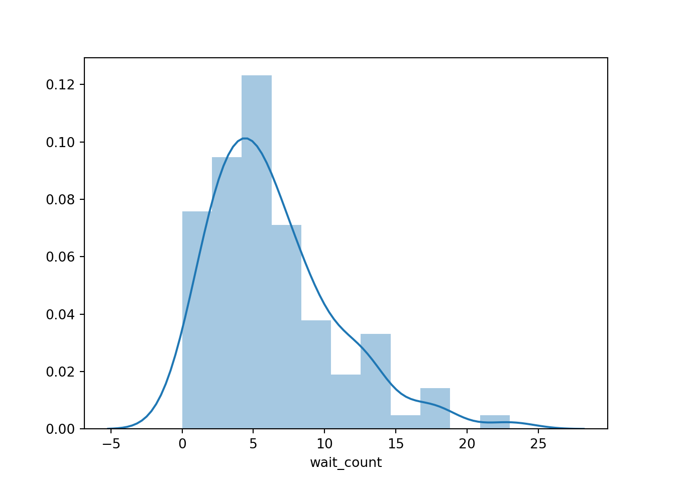
Generally less than half of all patients have to wait at all, but to see nice graphs of the wait time and close time, we need to get out of datetime format by applying total_seconds and dividing by 60 to convert to minutes.
sns.distplot(first_sim.results.avg_wait_time.dt.total_seconds().div(60))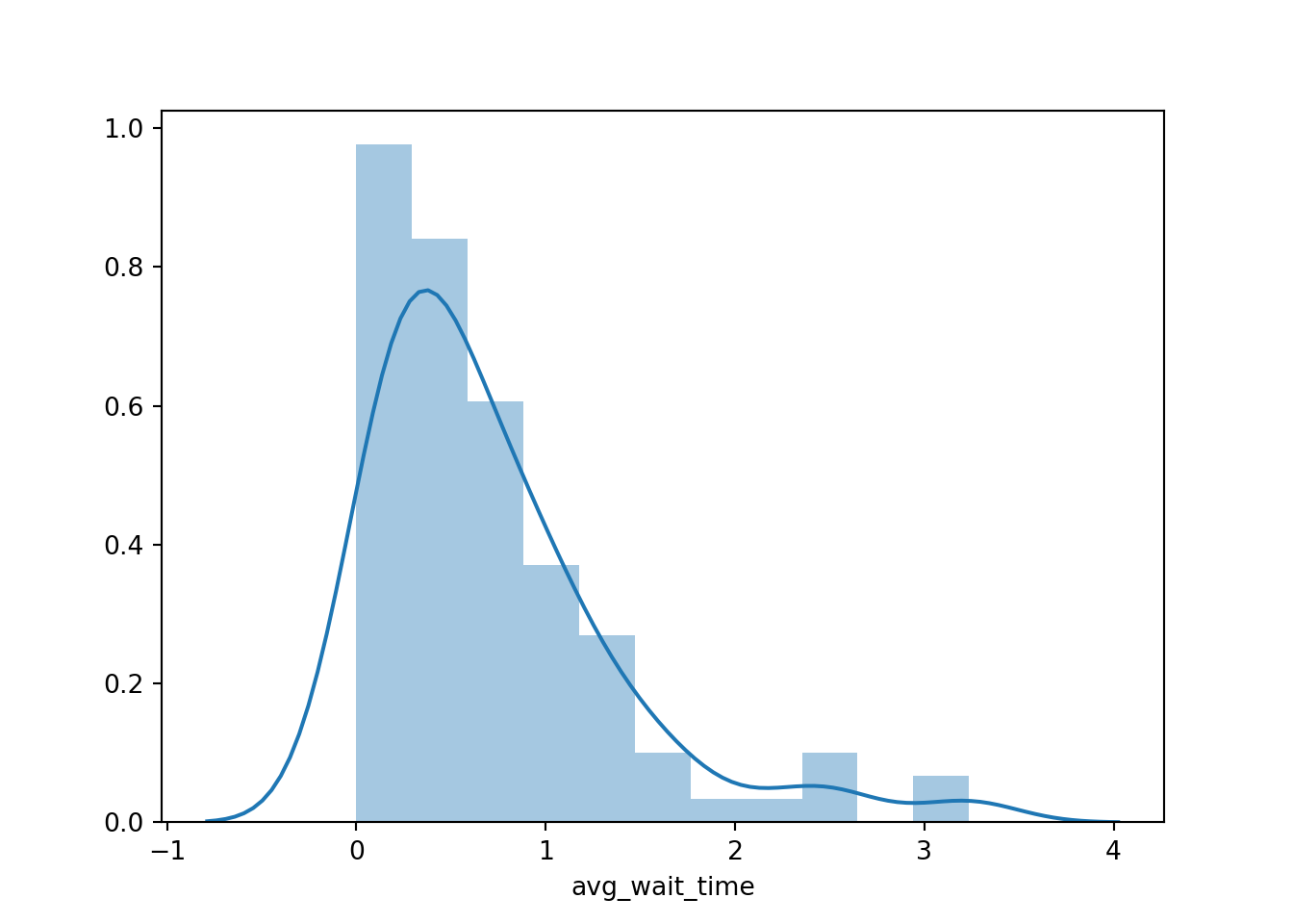
Similarly, we can plot the distribution of closing times as minutes after 4PM:
import datetime

sns.distplot((first_sim.results.close_time-datetime.datetime.combine(datetime.date.today(),datetime.time(16,0,0))).dt.total_seconds().div(60))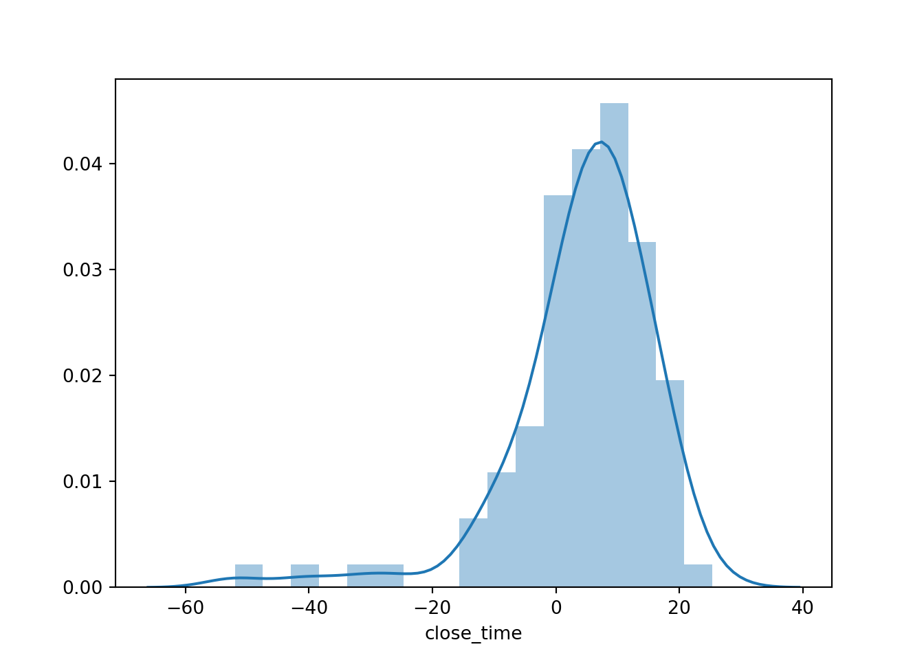
The negative times mean doctors were available to see patients, but no new patients came between the last appointment end and 4PM.
Next, we should incorporate some realism into our simulation - doctors need some breaks and likely pauses between patients to maintain charts, but I’ll leave that as an exercise to the reader…