One of the first things I learned studying abstract mathematics was that having non-examples were as important as examples of abstract structure. For instance, the definition of a group and some examples of groups it really only part of the picture - having examples of sets that satisfy all but one of the requirements to be a group allows you to see how the pieces fit together and lays a foundation for more solid intuition for further study.
When you start doing probabilistic programming or Bayesian modeling, you quickly encounter traceplots as a major diagnostic tool. However, neither Stan or PyMC3 provide good documentation about how to read them or what problems to look out for - at best you get vague references to fuzzy caterpillars. If your well versed in the theory of MCMC sampling you may not need such a practical guide to what a bad traceplots looks like, but as these tools become more popular and building Bayesian models becomes easier I think there’s a need for more non-examples of models - or examples of bad traceplots. Hopefully some find this useful.
Before we get started, I want to re-iterate the often repeated advice about Bayesian modeling: if diagnostics show problems, it’s often a problem with the model, not a simple change of settings in something like PyMC3 or Stan. Carefully think about your model and be open to reformulation.
How Bayesian Models Go Bad
Before getting into bad traceplots (and other diagnostics), let’s start with an overview of how things can go wrong with Bayesian models. First, your MCMC sampling can fail to converge, or diverge, which is a very bad thing. Second, our chains can converge, but fail to adequately explore the parameter space. This is often harder to detect and is the subject of Thomas Wiecki’s post linked to in the previous section. This post will focus on actual divergences (which are also an exploration failure, but usually more obvious) to highlight the signs of problems in traceplots.
To get an idea of divergence, think of the standard normal distribution. If you wanted to sample from a population that had such a distribution, you would want most of you samples to be between -2 and 2 (i.e. 2 standard deviations from the mean) - this is what is often called the ‘typical set’. Having most of your sample data in this range would allow you to clearly see the normal distribution. In higher dimensions, this is harder to do because the locations with high density (near the mode) that contribute to expectations have very low volume compared to tails in every other neighborhood with almost no density. In these higher dimensional settings, the typical set balances the high density/low volume near the mode with the low density/high volume ‘tails’ of our distribution. The goal of MCMC sampling is to compute our posterior distribution (or expectations using it). MCMC is a procedure that allows us to draw samples and refine how the next sample is drawn. If we start with a value far from the typical set, our next draw should get closer to the typical set, and so on. This is why there is a ‘burn-in’ or ‘tuning’ in MCMC sampling, we have to start at a random place and run our sampling until we (hopefully) get into the typical set, then the part of the chains we care about should be exploring the typical set. With a 1-dimensional normal distribution, this is easy and fast. But complex models may have a typical set that exists as a low dimensional space inside a much larger ambient space - Betancourt’s images of a 2-d loop in a plane is an easy visual and the smallest case where things get interesting. If we start far from the loop, we have to burn-in or tune our chains long enough that they at least find the loop. Divergence is failing to find the loop or only finding part of the loop. If were are able to find and explore most of the typical set, we may not get warnings or errors out of our sampler but will have biased samples, hence the need to know what problems to look for. If PyMC3 gives warnings about diverging chains, the simplest thing to try is increase the tune value, but if you have a bad model this can’t do much. Also, you should be tuning and sampling for as long as you can - running MCMC for arbitrarily short periods is asking for trouble.
The Model
To see examples of bad traceplots, we need a model. A decent one happens to be a small variation on the baseball batting average example. This tries to use data from the first part of the season to estimate batting performance for players of the rest of the season, and showed (among other things) that early season performance isn’t a great indicator of overall performance. Since I know almost nothing about baseball, my variation is looking at soccer penalty kicks. Rather than being interested in early estimates of season performance, I wanted to have a way of addressing the question of ‘Should player X be taking a penalty?’ or ‘Player x has missed all recent penalties, so shouldn’t someone else be taking them?’ (if you follow soccer, ‘player X’ was most recently Paul Pogba - but the same dialog occurs whenever a high profile player fails to score a penalty).
Scoring from a penalty should be well modeled by a binomial distribution, which requires a probability of success \(\theta\). This value must be between 0 and 1, so a hierarchical model with a Beta prior on \(\theta\). The particular Beta is determined by both a uniform random \(\phi\) that is a factor shared by all players (the global average of scoring a penalty) and \(\kappa\) that represents the variation among players. Having both the \(\phi\) and \(\kappa\) terms make this a ‘partial pooling’ instance as opposed to ‘no pooling’ (all players have an independent \(\theta\)) and ‘complete pooling’ with one \(\theta\) value that controls the entire group. I’ll keep my model that same as the baseball example except for the observed data and use a Pareto distributed \(\kappa\). Instead of pm.Pareto('kappa', m=1.5), we’ll use a transformed exponential distribution since the PyMC3 docs say it’s easier on the sampler (and we’re already going to give it problems).
import pymc3 as pmimport numpy as np
import matplotlib.pyplot as plt
import pandas as pd
import theano.tensor as tt
df = pd.read_csv('../../static/files/penalty_data.csv', encoding='latin-1')
score_cnt = df[['Player', 'Scored']].groupby('Player')['Scored'].apply(lambda x: sum(x=='Scored'))
total = df[['Player','Scored']].groupby('Player')['Scored'].agg(Total='count')
df2 = pd.concat([score_cnt, total], axis=1).reset_index()
#The PyMC3 part, finally
N = len(df2)
with pm.Model() as pk_model:
phi = pm.Uniform('phi', lower=0.0, upper=1.0)
kappa_log = pm.Exponential('kappa_log', lam=1.5)
kappa = pm.Deterministic('kappa', tt.exp(kappa_log))
thetas = pm.Beta('thetas', alpha=phi*kappa, beta=(1.0-phi)*kappa, shape=N)
y = pm.Binomial('y', n=df2['Total'], p=thetas, observed=df2['Scored'])One of our goals is to determine if a player who misses a few penalties is ‘anomalous’, so we want to add in this new player with no observed successes in 2 attempts.
with pk_model:

    theta_new = pm.Beta('theta_new', alpha=phi*kappa, beta=(1.0-phi)*kappa)
    y_new = pm.Binomial('y_new', n=2, p=theta_new, observed=0)
With our model in place, let’s move on to the sampling (and the problems).
Divergences
We build a model (or really just re-purposed one that didn’t have problems), so we’re all set to do inference and have nothing to worry about. In PyMC3 we’ll press the magic inference button and …
with pk_model:
    trace = pm.sample(500, progressbar=False)
Diverging chains! (I’ve suppressed the output, but you’ll see the counts below)
Whenever chains diverge, don’t fall into the trap of trying to justify them away - even one diverging chain among 1000 can be bad. To fix things we can (a) increase tuning, (b) increase target_accept, or (c) change our model. The first two are just sample parameters, so they’re easy but often won’t address the real problem (a bad model or bad data). Here I’ll note the number and percent of diverging chains to see how we improve.
diverging = trace['diverging']
print('Number of Divergent Chains: {}'.format(diverging.nonzero()[0].size))
## Number of Divergent Chains: 141diverging_perc = diverging.nonzero()[0].size / len(trace) * 100
print('Percentage of Divergent Chains: {:.1f}'.format(diverging_perc))## Percentage of Divergent Chains: 28.2Since I promised bad traceplots, let’s see our first:
pm.traceplot(trace, var_names=['phi', 'kappa'])## array([[<matplotlib.axes._subplots.AxesSubplot object at 0x7fb65ddd4310>,
## <matplotlib.axes._subplots.AxesSubplot object at 0x7fb65db5b910>],
## [<matplotlib.axes._subplots.AxesSubplot object at 0x7fb65cf1d9d0>,
## <matplotlib.axes._subplots.AxesSubplot object at 0x7fb65d9f0810>]],
## dtype=object)plt.show()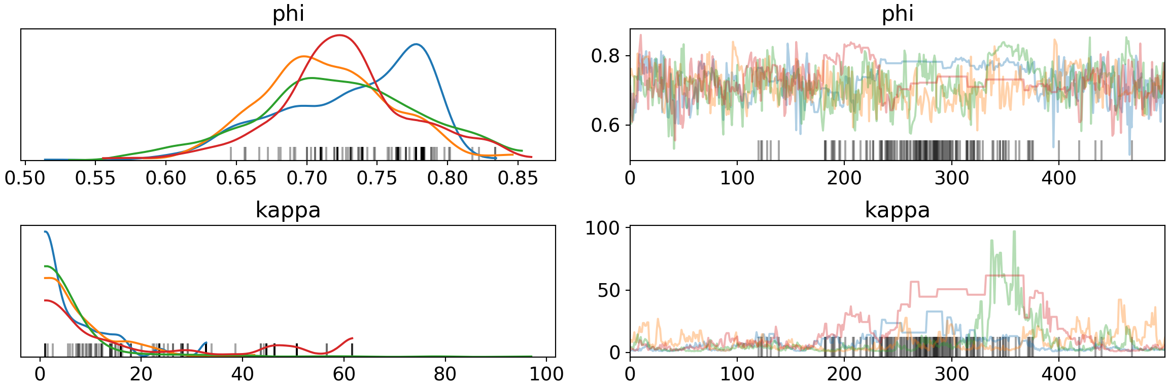
There are definitely variations in the chains for both phi and kappa (left) rather than the consistent convergence with expect. The ‘fuzzy caterpillars’ on the right clearly show chains getting stuck (flat, step-function like behavior) for both variables (the blue line of phi near the divergence marks), especially kappa. There are also 48 distributions for theta (one for each player) that we could look at (but this will take a long time to draw, so we won’t).
More Tuning
Let’s rebuild the trace with higher tuning to see if this improves things, I keep the tune and draw values intentionally on the low side to make problems obvious. I’ll report the number and percent of diverging chains as before.
with pk_model:
  trace = pm.sample(500, tune=1500, progressbar=False)
diverging = trace['diverging']
print('Number of Divergent Chains: {}'.format(diverging.nonzero()[0].size))## Number of Divergent Chains: 7diverging_perc = diverging.nonzero()[0].size / len(trace) * 100
print('Percentage of Divergent Chains: {:.1f}'.format(diverging_perc))## Percentage of Divergent Chains: 1.4pm.traceplot(trace, var_names=['phi', 'kappa'])## array([[<matplotlib.axes._subplots.AxesSubplot object at 0x7fb65df35d10>,
## <matplotlib.axes._subplots.AxesSubplot object at 0x7fb65e68cf50>],
## [<matplotlib.axes._subplots.AxesSubplot object at 0x7fb6625a53d0>,
## <matplotlib.axes._subplots.AxesSubplot object at 0x7fb65e8fe850>]],
## dtype=object)plt.show()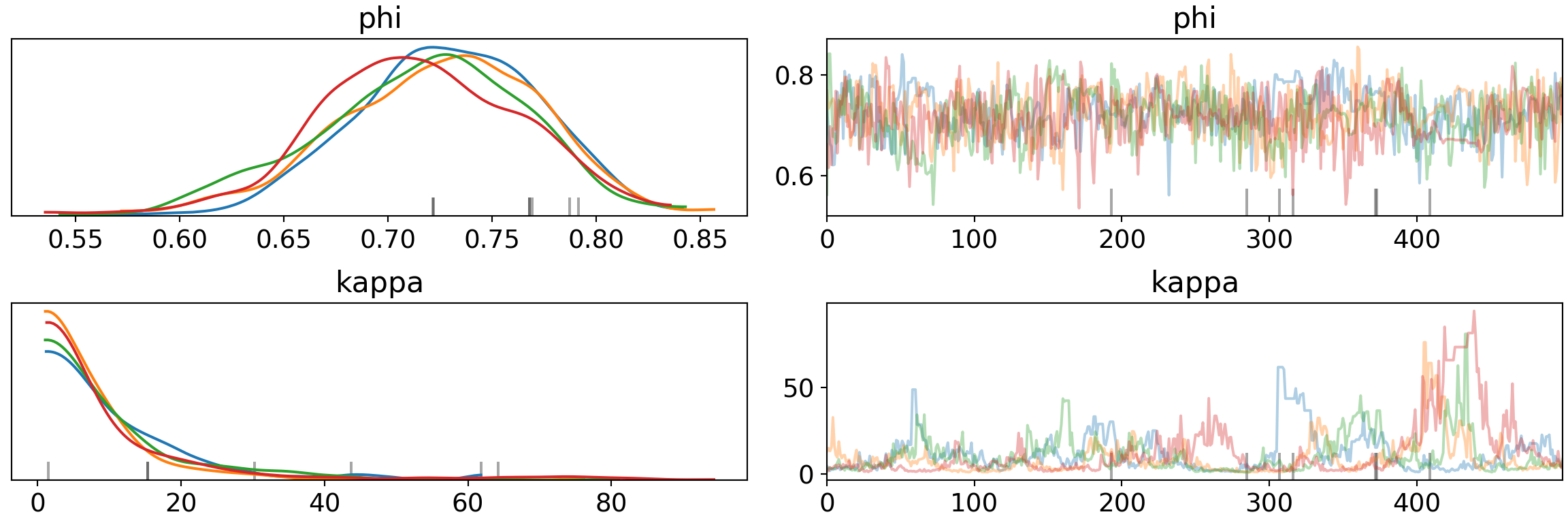
Increasing the number of tuning steps can shrink the divergences and improve the traceplots, but isn’t gauranteed to eliminate them (and can make problems more noticable at times). Increasing the sample size also gives a slight improvement, but makes problems harder to spot. On to target_accept.
Target Acceptance
By default, PyMC3 uses NUTS which does Hamiltonian Monte Carlo (HMC), which is basically Metropolis-Hastings with some significant performance boosts. In all of these, a sample is drawn and a random decision is made whether to keep or reject the sample. The long-term acceptance rate is the integrator step size of the algorithms and plays a crucial role in efficiency. High target acceptance means little to no rejection sampling, so you may be very inefficient at exploring your parameter space. The Stan development team (creators of NUTS) showed that anything between \(0.6\) and \(0.9\) were essentially equivalent to the optimal target acceptance in this paper, p. 14 and then both Stan and PyMC3 decided to use \(0.8\) as the default. Having an actual acceptance ratio above the target isn’t bad (you’ll get a warning in PyMC3, but it’s usually not cause for concern), but when we’re getting divergences after tuning we can reduce the amount of rejected samples to more thoroughly explore the space. Th rejection sampling helps keep us from taking too large of steps and diverging out to infinity, missing the typical set, or missing important features of the typical set.
Let’s see the impact of \(0.9\), before and after increased tuning.
with pk_model:
trace = pm.sample(500, tune=500, target_accept=0.9, progressbar=False)
diverging = trace['diverging']
print('Number of Divergent Chains: {}'.format(diverging.nonzero()[0].size))
## Number of Divergent Chains: 35diverging_perc = diverging.nonzero()[0].size / len(trace) * 100
print('Percentage of Divergent Chains: {:.1f}'.format(diverging_perc))## Percentage of Divergent Chains: 7.0pm.traceplot(trace, var_names=['phi', 'kappa'])## array([[<matplotlib.axes._subplots.AxesSubplot object at 0x7fb65c5b2490>,
## <matplotlib.axes._subplots.AxesSubplot object at 0x7fb65e55df10>],
## [<matplotlib.axes._subplots.AxesSubplot object at 0x7fb65eb927d0>,
## <matplotlib.axes._subplots.AxesSubplot object at 0x7fb65dafab10>]],
## dtype=object)plt.show()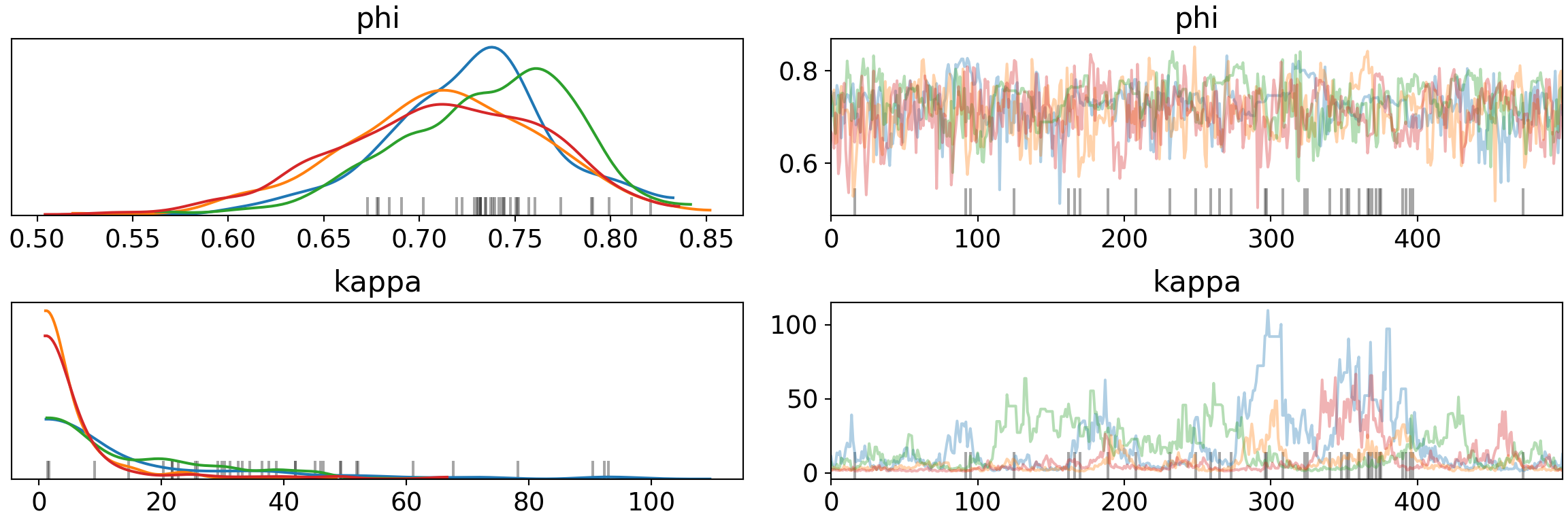
With increased tuning also:
with pk_model:
  trace = pm.sample(500, tune=1500, target_accept=0.9, progressbar=False)
diverging = trace['diverging']
print('Number of Divergent Chains: {}'.format(diverging.nonzero()[0].size))## Number of Divergent Chains: 10diverging_perc = diverging.nonzero()[0].size / len(trace) * 100
print('Percentage of Divergent Chains: {:.1f}'.format(diverging_perc))## Percentage of Divergent Chains: 2.0pm.traceplot(trace, var_names=['phi', 'kappa'])## array([[<matplotlib.axes._subplots.AxesSubplot object at 0x7fb65e2aced0>,
## <matplotlib.axes._subplots.AxesSubplot object at 0x7fb65c6d0490>],
## [<matplotlib.axes._subplots.AxesSubplot object at 0x7fb65bcd5410>,
## <matplotlib.axes._subplots.AxesSubplot object at 0x7fb65e63ed50>]],
## dtype=object)plt.show()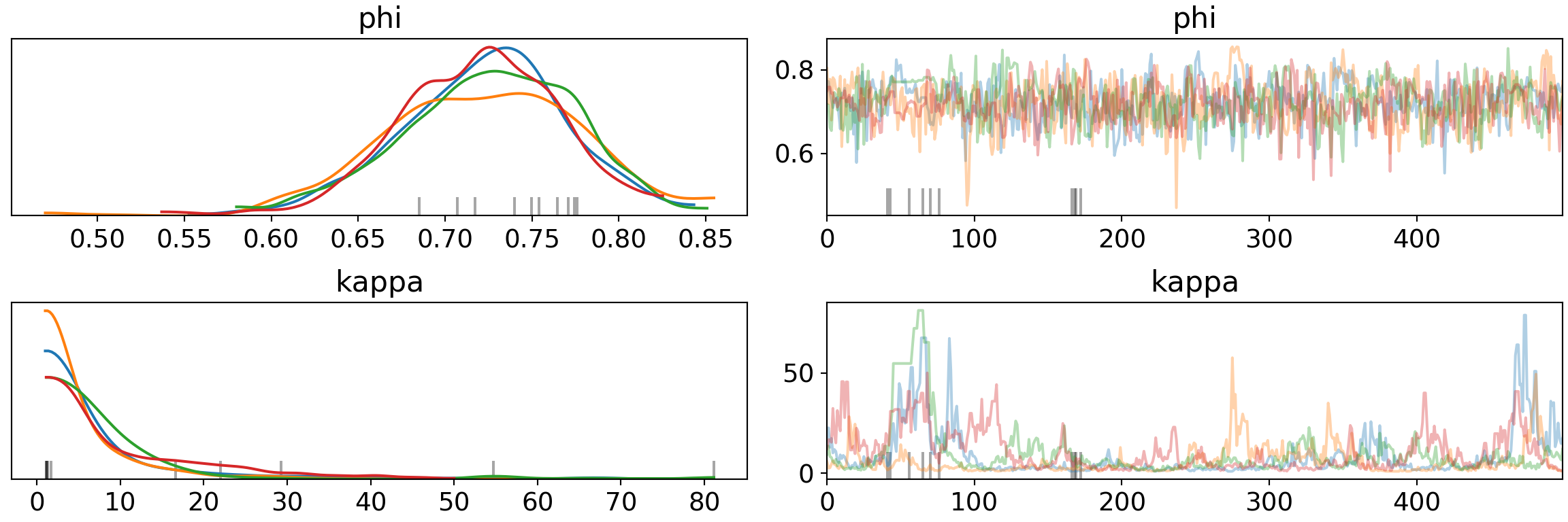
Both more tuning and increasing target_accept reduce divergence separately, but the effects don’t necessarily combine. Part of this is due to the model/data we have - we’re trying to do inference with 1 or 2 observations in many cases.
Proper Exploration
When chains diverge, we’re told to ‘increase target_accept or reparameterize’ by the all knowing computer. The task of reparameterization is more involved, but can also us to handle more subtle problems like failing to explore the parameter space without having true divergence occurring. Osvaldo Martin gives a nice overview of what reparameterization means here, with the key idea being to find an equivalent model that’s easier to work with computationally - i.e. easier for MCMC to explore. Thomas Wiecki has a nice blog post showing how subtle exploratory failure can look and how to use a non-centered hierarchical model to reparameterize.
For our penalty kick model, we have an obstacle of very few observations for most of our players, but this is a problem in real life - we rarely have ‘ideal’ data. To make an equivalent model we can try (a) more informative priors, (b) continuous approximations to discrete distributions, and then move to more substantive changes if needed.
A more informative prior on \(\phi\) is very reasonable. Recall that \(\phi\) is a factor shared by all players and relates to how likely a player is to score a penalty. Our prior puts no restriction on \(\phi\) other than that it must be between 0 and 1, but if a player was generally unlikely to score a penalty it would make for a very poor reward for a foul committed near the goal. It’s reasonable to assume that \(\phi\) is above \(0.5\), but we’ll maintain the uniform distribution and upper bound. The Pareto distribution on kappa is good for batting averages (most players will have low averages, but some will be very high), but this is also dependent on the number of ‘at bats’, which is typically several times per game. This is almost the reverse for penalty kicks where a save or miss is more equivalent to getting a hit in baseball and most players will only take 1-3 penalty kicks (in league games only, no shoot-outs) during an entire season. Perhaps a normal with wide variation would be better than a Pareto. Since we can’t have negative values on kappa, we’ll use a TruncatedNormal. This constricts the parameter space considerably.
with pm.Model() as pk_model2:

    phi = pm.Uniform('phi', lower=0.5, upper=1)
    kappa = pm.TruncatedNormal('kappa', mu=3, sigma=2, lower=0)

    thetas = pm.Beta('thetas', alpha=phi*kappa, beta=(1.0-phi)*kappa, shape=N)
    y = pm.Binomial('y', n=df2['Total'], p=thetas, observed=df2['Scored'])

    theta_new = pm.Beta('theta_new', alpha=phi*kappa, beta=(1.0-phi)*kappa)
    y_new = pm.Binomial('y_new', n=2, p=theta_new, observed=0)

    trace2 = pm.sample(500, tune=1500, target_accept=0.9, progressbar=False)
diverging = trace2['diverging']
print('Number of Divergent Chains: {}'.format(diverging.nonzero()[0].size))## Number of Divergent Chains: 0diverging_perc = diverging.nonzero()[0].size / len(trace2) * 100
print('Percentage of Divergent Chains: {:.1f}'.format(diverging_perc))## Percentage of Divergent Chains: 0.0No more divergences. Our traceplot reveals the exploration that we hope from good MCMC sampling without steps, oscillations, pinching, fly-aways, or other signs of problems.
pm.traceplot(trace2, var_names=['phi', 'kappa'])## array([[<matplotlib.axes._subplots.AxesSubplot object at 0x7fb65dd07950>,
## <matplotlib.axes._subplots.AxesSubplot object at 0x7fb65b480210>],
## [<matplotlib.axes._subplots.AxesSubplot object at 0x7fb65b61f510>,
## <matplotlib.axes._subplots.AxesSubplot object at 0x7fb65b54fe90>]],
## dtype=object)plt.show()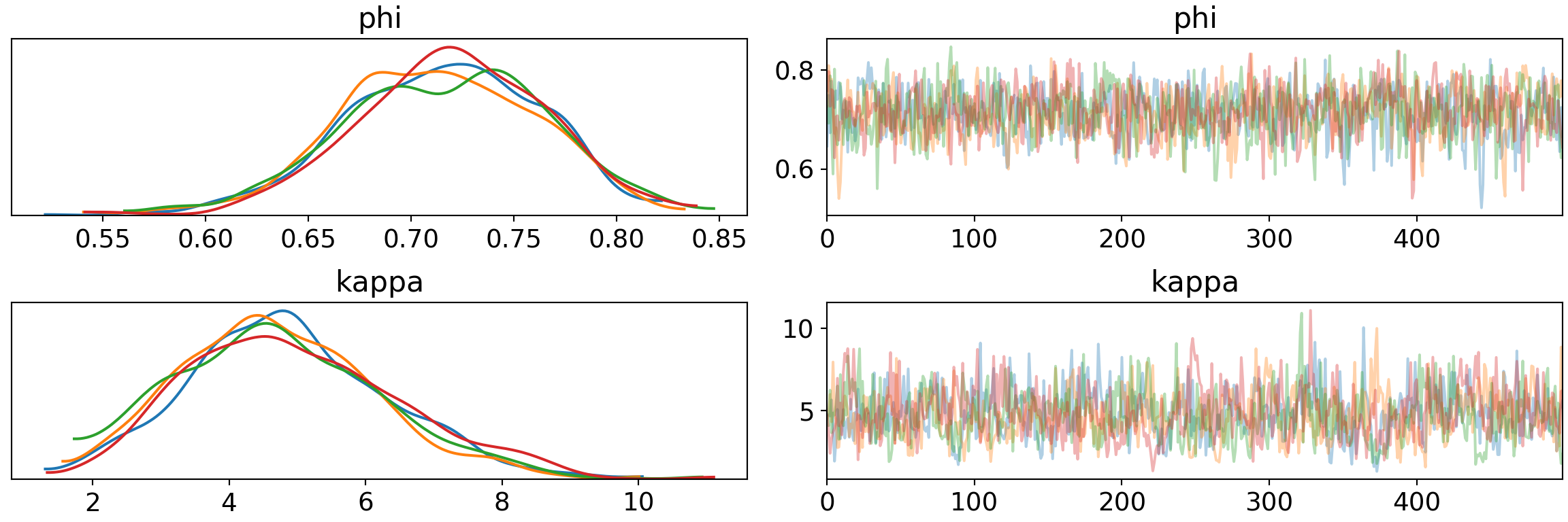
Since we know have a model that seems like it works, we can look at the probability of success of our player who has missed his first 2 penalties.
pm.traceplot(trace2, var_names=['theta_new'])## array([[<matplotlib.axes._subplots.AxesSubplot object at 0x7fb65b4f47d0>,
## <matplotlib.axes._subplots.AxesSubplot object at 0x7fb65b415910>]],
## dtype=object)plt.show()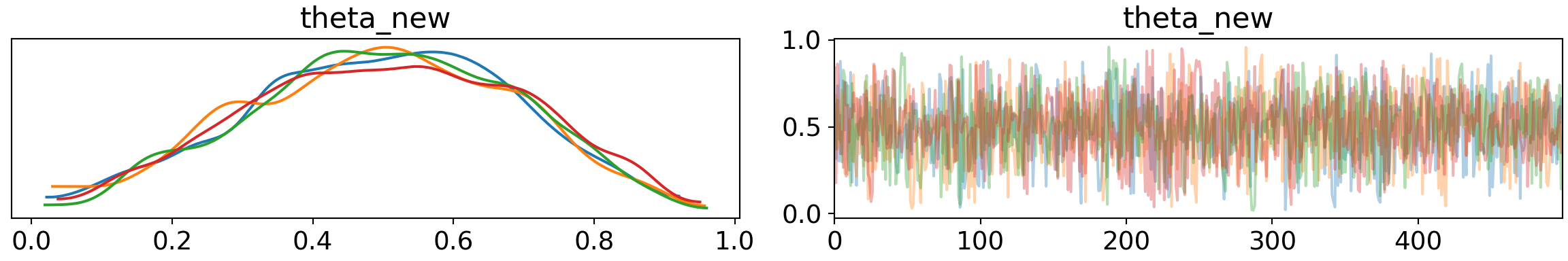
pm.plot_posterior(trace2, var_names=['theta_new', 'phi'])## array([<matplotlib.axes._subplots.AxesSubplot object at 0x7fb65b41a6d0>,
## <matplotlib.axes._subplots.AxesSubplot object at 0x7fb65b3cad50>],
## dtype=object)plt.show()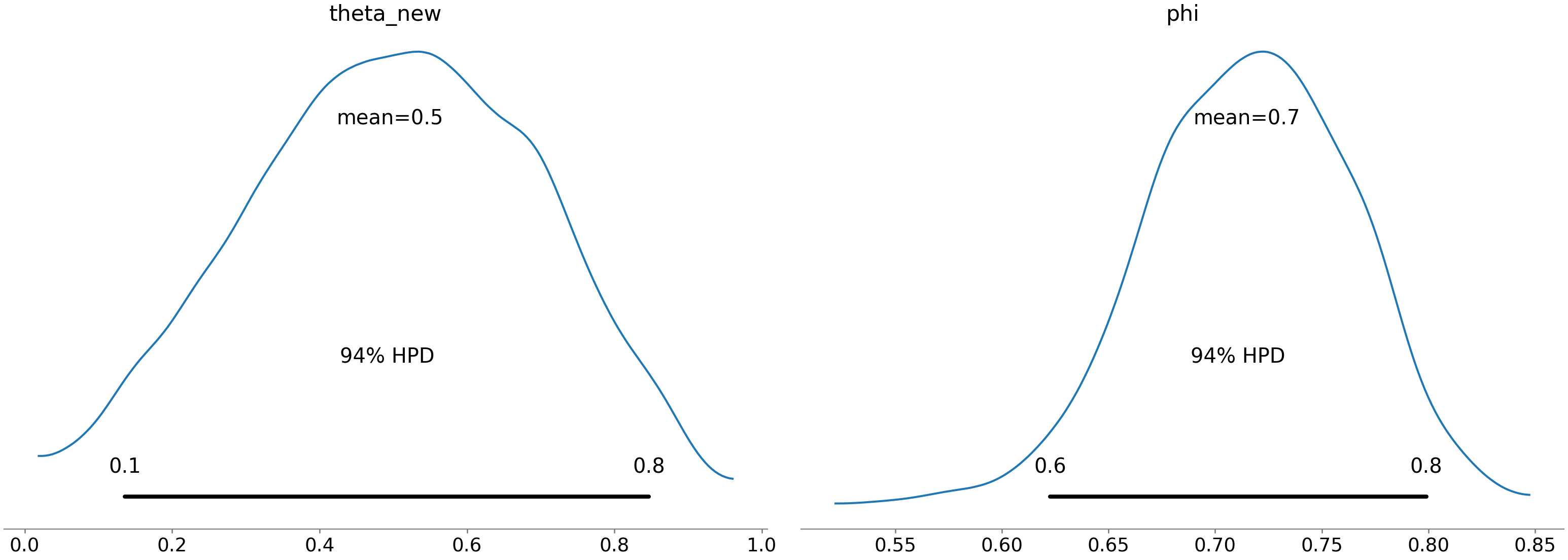
The player’s performance allows for theta to be very low, but could be in line with the global average. Comparison will all players shows overlap on the high end with all players, so this is likely just a patch of poor performance or an area to work on in training than a true deficiency.
Additional Plots
Besides traceplots, PyMC3 and Arviz can produce a wide variety of plots to visualize Bayesian models. Like traceplots, each focuses on a particular aspect of MCMC sampling or Bayesian inference so they have different uses. A good model should consistently show good plots, but a bad model may have a decent traceplot but bad energy plot. As with exploratory data analysis, don’t look at just one plot or one diagnostic feature - especially if you’re doing something important like trying to determine penalty kick performance.